Calculate drag force against a cyclist using MATLAB.

- 1. Aim: To write a program to find the variation of Drag force when compared to different values of Velocity and Coefficient of Drag.

- 2. Objectives:

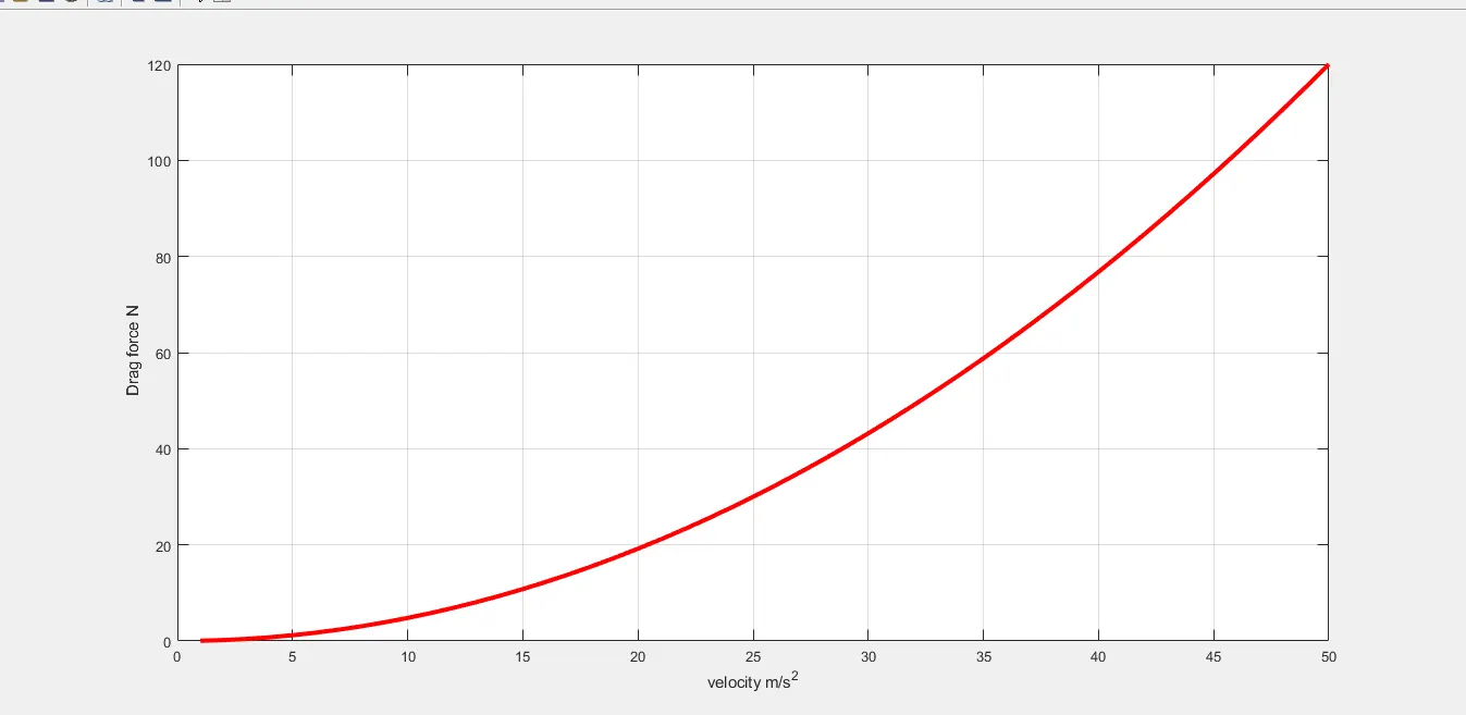
- To generate the plot of Velocity vs Drag force.

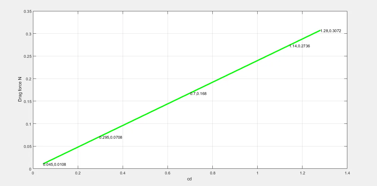
- To generate the plot of Coefficient of Discharge vs Drag force.

- Understanding the change in Drag force corresponds to Velocity and Coefficient of drag.

- 3. Method:

- 3.1 The program shown below is the way we can compare the variation of drag force compared with different values of velocity and drag force.

% This is a program to find drag force. Here the velocity is changing and all other parameters are constant 
% rho = density of air in kg/m^3
% a =  frontal area in m^2
% v = velocity in m/s
% cd = drag coefficient

cd = 0.8
a = 0.1 
v = [1:50];
rho = 1.2 
Drag_force = 0.5*cd*rho*a*v.^2;
plot(v,Drag_force,'color','r','linewidth',3)
xlabel('velocity m/s^2')
ylabel(' Drag force N')
grid on

- Drag Coefficient is a non-dimensional quantity and it has no uni.

- Velocity here is a row vector i.e it has a row and number of a column. For each value of velocity, we are going to calculate drag force and going to plot a graph of velocity vs Drag force.

- V here is a matrix and we need to use an element-wise operator so in the formula it is v.^2.

- As we have taken the velocity values from 1 to 50, the curve will come smoother and a parabolic one.

- As velocity v is changing Drag force is going to change proportional to v^2 i.e if we increase the velocity 2 times drag will change by 4 times. Means we are able to travel 2 times faster drag force will be 4 times more which means fuel economy will drop accordingly.

- 'color' is a command used to give a colour to the plot and 'r' here represents the Red colour.

- To improve the appearance of the plot 'linewidth' command is used, which basically increases the thickness of the plot.

Plot showing the variation of Drag force w.r.t velocity.

-3.2 The program given below is representing the behaviour of the drag force compared with the different values of the coefficient of drag.

% This is a program to find drag force. Here the Coefficient of drag is
% changing for same frontal area but different shapes.
% rho = density of air in kg/m^3
% a =  frontal area in m^2
% v = velocity in m/s
% cd = drag coefficient

cd = [0.045 0.295 0.7 1.14 1.28]
a = 0.1 
v = 2
rho = 1.2 
Drag_force = 0.5*cd*rho*a*v^2;
plot(cd,Drag_force,'color','g','linewidth',3)
xlabel('cd ')
ylabel(' Drag force N')
grid on

- From the plot, it can be seen that as the value of Coefficient of drag changing the drag force is varying accordingly.

- Here from the graph, it is appearing as the drag force is changing linearly with the coefficient of drag.

- Drag coefficient values are taken from the internet and the image is shown below.

Plot showing Drag force vs Coefficient of drag.

4. Learning outcome:

- Plotting the variation of drag force with respect to velocity.

- Plotting the variation of drag force with respect to the coefficient of drag.

- Understanding the behaviour of drag force w.r.t velocity and coefficient of drag.

5. Conclusion:

- From the 1st graph, velocity vs drag force, it can be seen that the behaviour of the drag force is parabolic. For each value of velocity, drag force is changing by a proportion of v^2.

- For the 2nd graph, coefficient of drag vs drag force, in this case, the variation is linear and the plot comes as a straight line.