Flow over a cylinder

Aim:-

To simulate the flow over a cylinder for the conditions shown in the video. To start, run a baseline simulation and then calculate the Reynolds number. Then increase the Reynolds number by a factor of 20%, 40%, and 100% then run the transient flow simulation.

Objective:

1. Calculate the Reynolds number for different inlet velocity.
2. Perform flow simulation on a cylinder with different inlet velocity corresponding to their different Reynolds number.
3. Obtain velocity and pressure contour. Obtain pressure - velocity animation.
4. Compare the result and draw a conclusion.

Introduction:-

CFD is a branch of fluid mechanics that uses numerical analysis and algorithms to solve and analyse problems that involve turbulent fluid flows. It is widely accepted that the Navier–Stokes equations (or simplified Reynolds-averaged Navier–Stokes equations) are capable of exhibiting turbulent solutions, and these equations are the basis for essentially all CFD codes.

The Reynolds number is the ratio of inertial forces to viscous forces and is a convenient parameter for predicting if a flow condition will be laminar or turbulent. It can be interpreted that when the viscous forces are dominant (slow flow, low Re) they are sufficient to keep all the fluid particles in line, then the flow is laminar. Even exceptionally low Re indicates viscous creeping motion, where inertia effects are negligible. When the inertial forces dominate over the viscous forces (when the fluid is flowing faster and Re is larger) then the flow is turbulent.

Laminar flow. For practical purposes, if the Reynolds number is less than 2100, the flow is laminar. The accepted transition Reynolds number for flow in a circular pipe is Re_d,crit = 2300. Transitional flow. At Reynolds numbers between about 2100 and 4000, the flow is unstable as a result of the onset of turbulence. These flows are sometimes referred to as transitional flows. Turbulent flow. If the Reynolds number is greater than 4000, the flow is turbulent. Most fluid systems in nuclear facilities operate with turbulent flow.

The Reynolds number is defined as:

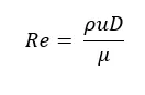
where:

• V is the flow velocity.
• D is the pipe diameter.
• ρ fluid density (kg/m³)
• μ dynamic viscosity (Pa.s)
• ν kinematic viscosity (m²/s); ν = μ / ρ

Procedure:-

1. Model the cylinder as per the given dimension below and save it.
2. Calculate the baseline Reynolds number by using the given parameters using the Reynolds Number formula, take the baseline Reynolds number as Re=13535.91.
3. Using this calculate the three Reynolds number by using 20%, 40%,100% of baseline Reynolds number.
4. Create a wizard and set the requires conditions like air medium, time-dependent, external flow and velocity.
5. Measure the computation domain and calculate the flow time and end time.
6. Insert the cut plot at the middle of the cylinder and show velocity and pressure plot for all the three Reynolds number.
7. Create an animation for both velocity and pressure plot for all the three values.

Geometric Parameters:-

• Diameter = 0.02 m.
• length = 0.05 m.
• rho = 1.225 kg/m³
• mu = 1.81 × 10^-5kg/(ms)

The fluid used = air.

For the baseline simulation, the velocity is 10 m/s.

For case 1 : v1 = 10m/s Flow Time 1 = 0.02s.

Re = (1.225 * 10 * 0.02) / (1.81 × 10^-5)

Re = 13535.9116

For case 2 : By increasing the Reynolds number by 20%, Re = 16243.09392

V2 = 12 m/s. Flow Time 2 = 0.03s.

For case 3: By increasing the Reynolds number by 40%, Re = 18950.27624

V3 = 14 m/s. Flow Time 3 = 0.025s.

For case 4: By increasing the Reynolds number by 100%, Re = 27071.8232

V4 = 20 m/s. Flow Time 4 = 0.018s

Results:-

For Case 1, Figure 1 and 2 shows the pressure and velocity plot.

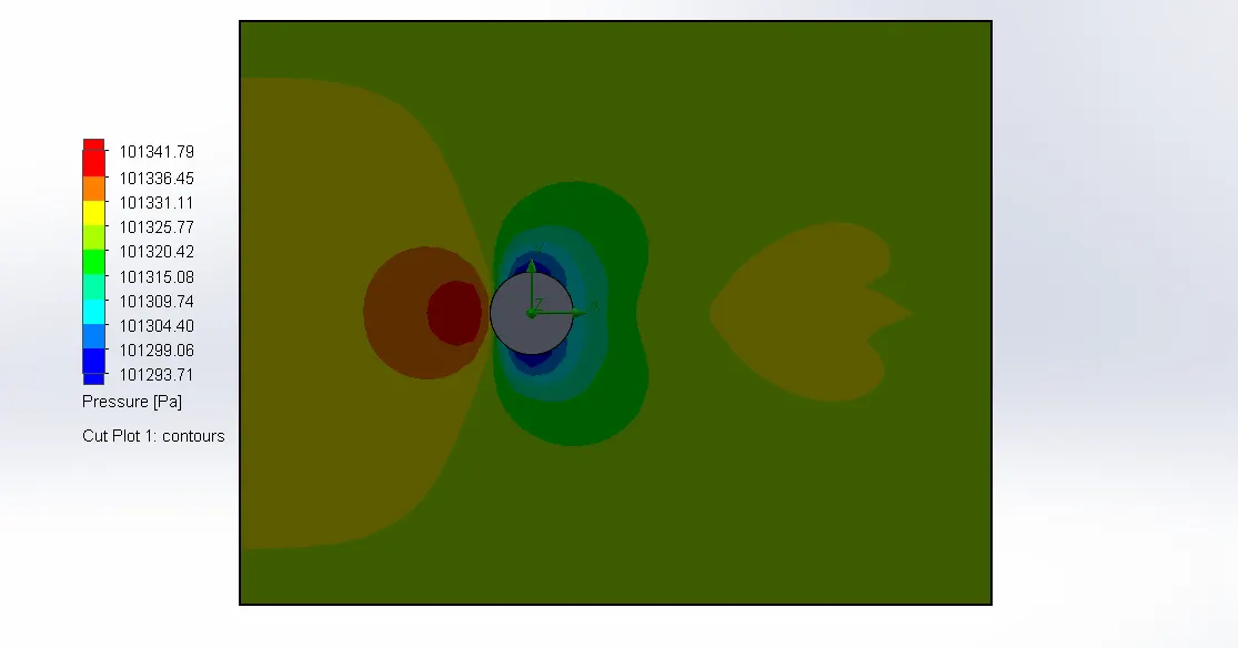
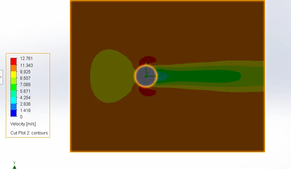
Figure 1: pressure plot for case 1 Figure 2: velocity plot for case 1

Youtube Link for the pressure plot for case 1 Youtube Link for the velocity plot for case 1

For Case 2, Figure 3 and 4 shows the pressure and velocity plot.

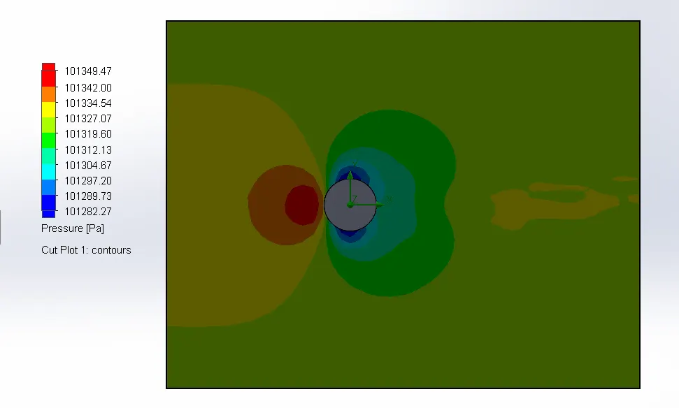
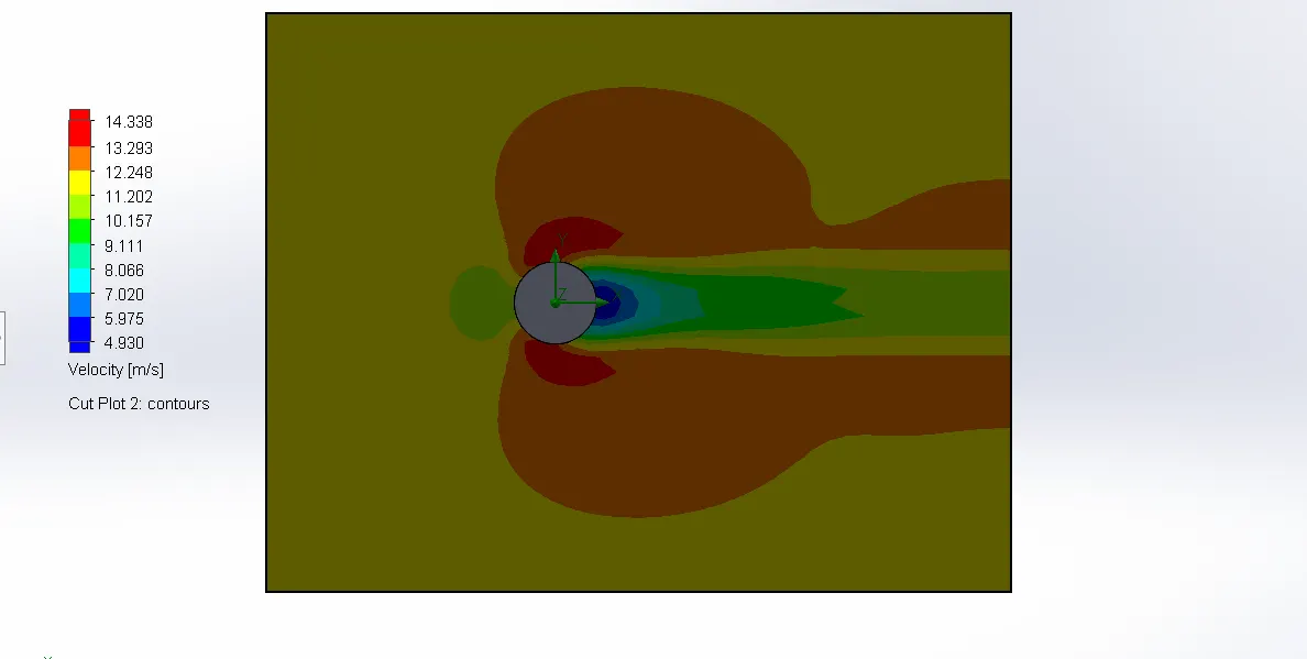
Figure 3: pressure plot for case 2 Figure 4: velocity plot for case 2

Youtube Link for the pressure plot for case 2 Youtube Link for the velocity plot for case 2

For Case 3, Figure 5 and 6 shows the pressure and velocity plot.

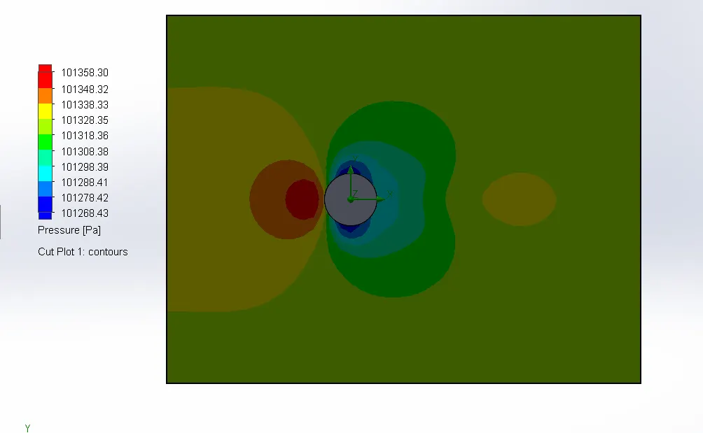
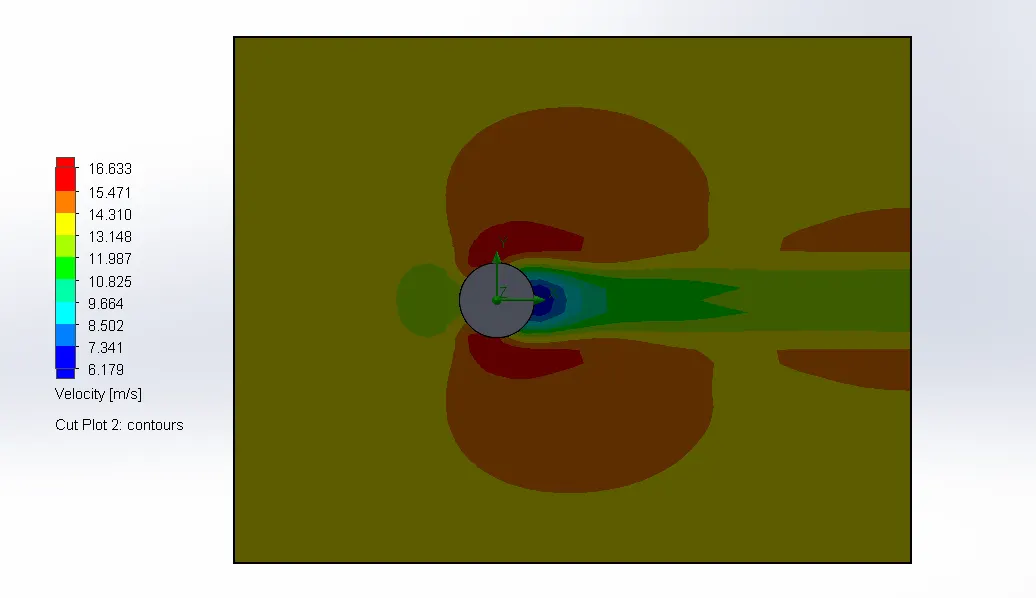
Figure 5: pressure plot for case 3 Figure 6: velocity plot for case 3

Youtube Link for the pressure plot for case 3 Youtube Link for the velocity plot for case 3

For Case 4, Figure 7 and 8 shows the pressure and velocity plot.

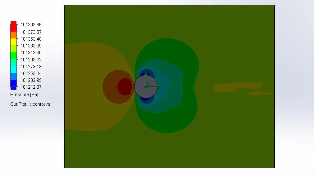
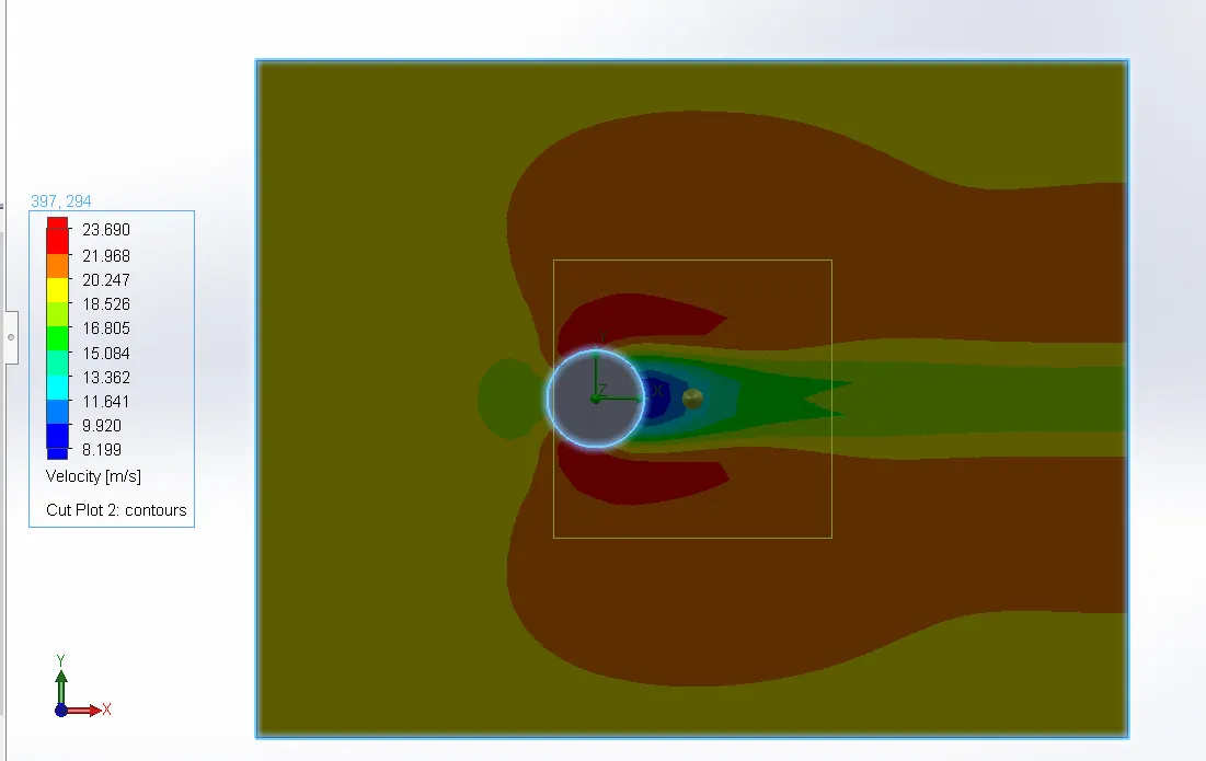
Figure 7: pressure plot for case 4 Figure 8: velocity plot for case 4

Youtube Link for the pressure plot for case 4 Youtube Link for the velocity plot for case 4

Conclusion:

When the air encounters cylinder surface due to the circular cross-section of the cylinder the air diverges and it leads to increase in pressure and velocity in that region but at the front and back portion in the linear direction the amount of air reaching decreases and the pressure and velocity decreases. This large region is formed due to flow separation creates the wake region, this region increases in size when the velocity of the air increases.In the wake region, the flow is highly unsteady and large eddies are formed which leads to high turbulence and producing drag, with an increase in velocity the turbulence also increases and so does drag.

References:-

• flow/#:~:text=In%20fluid%20dynamics%2C%20laminar%20flow,no%20disruption%20between%20the%20layers.
• https://www.reactor-physics.com/engineering/fluid-dynamics/reynolds-number/