Final Project: Design of an Electric Vehicle

Electric Vehicle:- 

a)Electric Vehicle is a vehicle that uses electric motors to produce power and a battery to store energy.

b) It uses an electric motor for propulsion and moving the vehicle instead of an internal combustion engine.

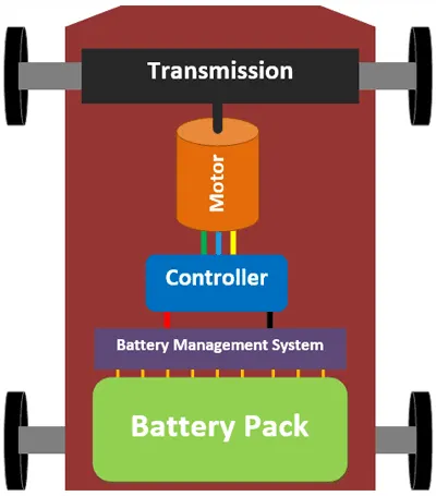
System level Block diagram of EV:-

    The electric vehicle consists of-

    a) Charging port- EV is charged through the charging port.

    b) Onboard charger- It acts as AC to DC rectifier.

    c) Battery- It stores the DC energy converted by an onboard charger.

    d) Power Controller- It controls the power required by the motor through the battery as a mediator and provides the power to the motor when needed. An inverter changes the DC power stored in the battery to AC.

    e) Motor - It produces the torque and supply power to rotate the wheel.

    f) Drivetrain - It contains a differential gearbox and fixed gear as the motor is capable of generating large variations of torque needed by the vehicle to run.

    g) Auxillary battery- To run the auxiliary components like headlight, wiper, etc.

    h) Thermal management system- To maintain the engine and cabin temperature.

    The losses to be considered while designing an electric powertrain are-

    Motor loss, Accessory loss, Charging loss, Inverter Loss, Mechanical losses.

- More Key components of electric Vehicle:

• Transmission system: Mechanical power is delivered from the motor shaft to the wheels.
• Traction motor: Propulsion power unit which generates motion from electric power.
• Inverter and controller: Changing both the type and extent of electrical power from the battery to the motor.
• Traction battery pack: Energy storage unit which makes energy expenditure while driving the vehicle and acquire energy while charging.

- Design of an Electric Vehicle:

Blocks used to design the model:

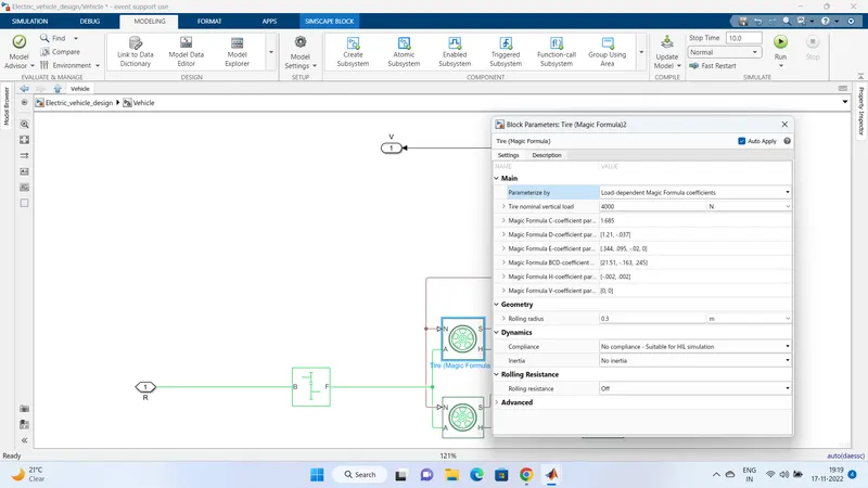
1) Tire:

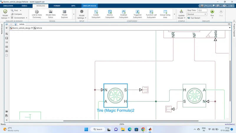
Represents the longitudinal behavior of a highway tire characterized by the tire Magic Formula. The block is built from Tire-Road Interaction (Magic Formula) and Simscape Foundation Library Wheel and Axle blocks. Optionally, the effects of tire inertia, stiffness, and damping can be included.

A - 

Connection A is the mechanical rotational conserving port for the wheel axle.

H- 

Connection H is the mechanical translational conserving port for the wheel hub through which the thrust developed by the tire is applied to the vehicle.

N-

Connection N is a physical signal input port that applies the normal force acting on the tire.

The force is considered positive if it acts downwards.

S-

Connection S is a physical signal output port that reports the tire slip.

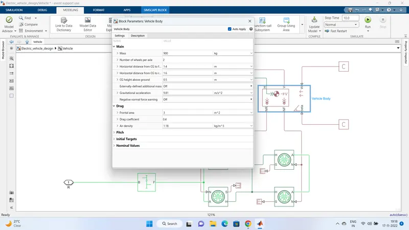
2) Vehicle Body:

Represents a two-axle vehicle body in longitudinal motion. The block accounts for body mass, aerodynamic drag, road incline, and weight distribution between axles due to acceleration and road profile. The vehicle can have the same or a different number of wheels on each axle. Optionally include pitch and suspension dynamics or additional variable mass and inertia. The vehicle does not move vertically relative to the ground.

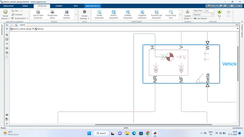
H-

Connection H is the mechanical translational conserving port associated with the horizontal motion of the vehicle body.

V-

vehicle velocity

Nf-

Front Wheel normal force

Nr-

Rear wheel normal force.

3) Simple Gear:

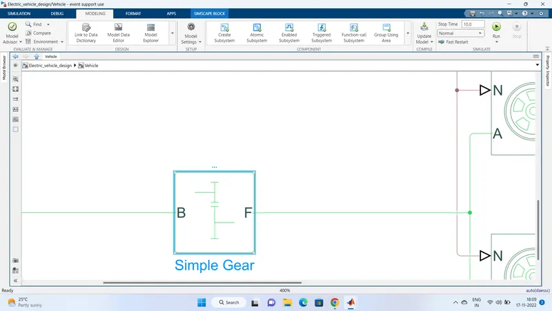
Represents a fixed-ratio gear or gearbox. No inertia or compliance is modeled in this block. You can optionally include gear meshing, backlash, and viscous bearing losses.

Connections B (base) and F (follower) are mechanical rotational conserving ports.

4) Constant and PS constant:

This block creates a physical signal constant:

y = constant

The Constant parameter accepts both positive and negative values. The block output is a physical signal port.

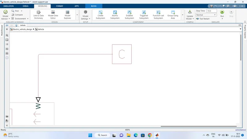
5) Connection port:

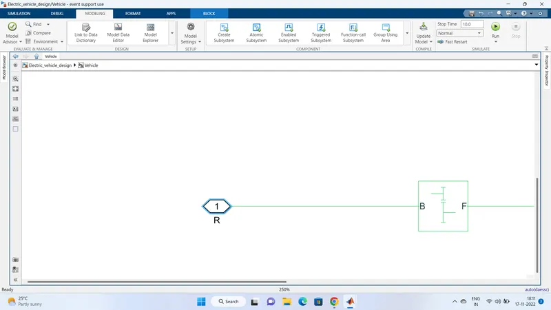
6) Drive Cycle Source:

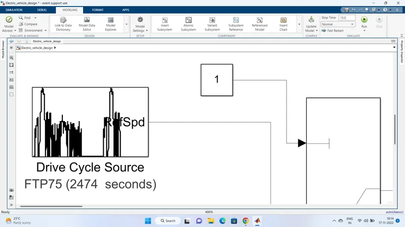
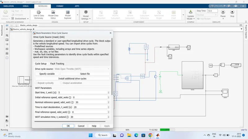
Generates a standard or user-specified longitudinal drive cycle. The block output is the vehicle longitudinal speed. You can import drive cycles from:

- Predefined sources

- Workspace variables, including arrays and time series objects

- mat, xls, xlsx, or txt files

Use the fault tracking parameters to identify drive cycle faults within specified speed and time tolerances.

7) Multiport Switch:

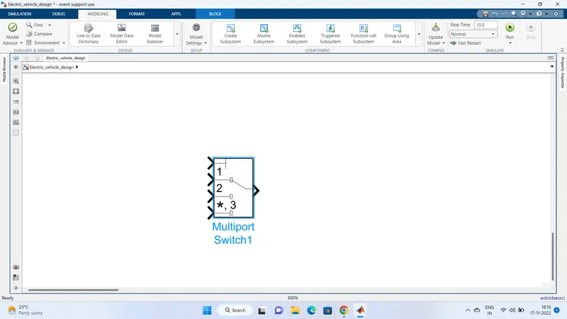
Pass through the input signals corresponding to the truncated value of the first input. The inputs are numbered top to bottom (or left to right). The first input port is the control port. The other input ports are data ports.

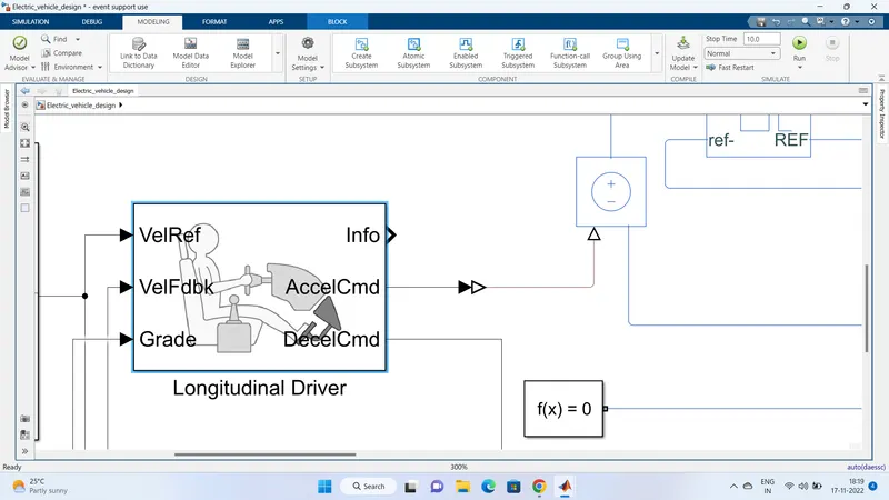
8) Longitudinal driver:

A parametric longitudinal speed tracking controller for generating normalized acceleration and braking commands based on reference and feedback velocities.

Use the external actions to input signals that can disable, hold, or override the closed-loop commands determined by the block. The block uses this priority for the input commands: disable, hold, override.

9) Controlled Voltage source:

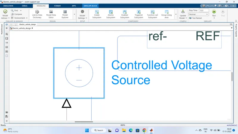
The block represents an ideal voltage source that is powerful enough to maintain the specified voltage at its output regardless of the current passing through it. The output voltage is V = Vs, where Vs is the numerical value presented at the physical signal port.

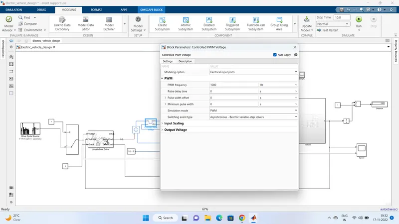
10) Controlled PWM Voltage:

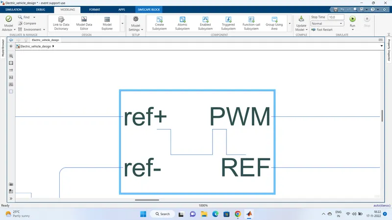
This block creates a Pulse-Width Modulated (PWM) voltage across the PWM and REF ports. The output voltage is zero when the pulse is low and is equal to the Output voltage amplitude parameter when high. The duty cycle is set by the input value. At time zero, the pulse is initialized as high unless the duty cycle is set to zero or the Pulse delay time is greater than zero.The Simulation mode can be set to PWM or Averaged. In PWM mode, the output is a PWM signal. In Averaged mode, the output is constant with a value equal to the averaged PWM signal.

11) H-Bridge:

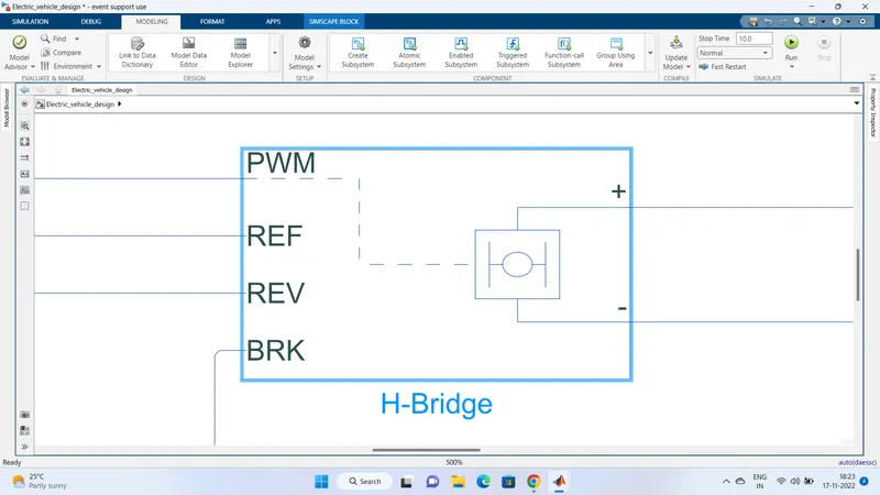
This block represents an H-bridge motor drive. The block can be driven by the Controlled PWM Voltage block in PWM or Averaged mode. In PWM mode, the motor is powered if the PWM port voltage is above the Enable threshold voltage. In Averaged mode, the PWM port voltage divided by the PWM signal amplitude parameter defines the ratio of the on-time to the PWM period. Using this ratio and assumptions about the load, the block applies an average voltage to the load that achieves the correct average load current. The Simulation mode parameter value must be the same for the Controlled PWM Voltage and H-Bridge blocks.

12) Current Sensor:

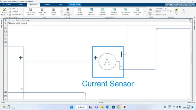
The block represents an ideal current sensor, that is, a device that converts current measured in any electrical branch into a physical signal proportional to the current. Connections + and - are conserving electrical ports through which the sensor is inserted into the circuit. Connection I is a physical signal port that outputs the current value.

13) Controlled Current Source:

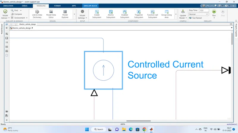
The block represents an ideal current source that is powerful enough to maintain the specified current through it regardless of the voltage across it. The output current is I = Is, where Is is the numerical value presented at the physical signal port.

14) Solver Configuration:

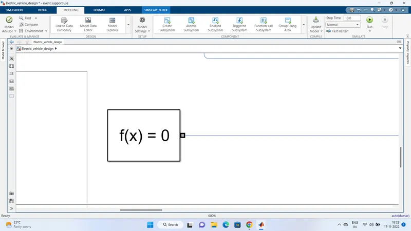
Defines solver settings to use for simulation.

15) Electrical Reference:

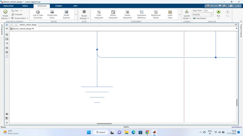
Electrical reference port. A model must contain at least one electrical reference port (electrical ground).

16) Battery: 

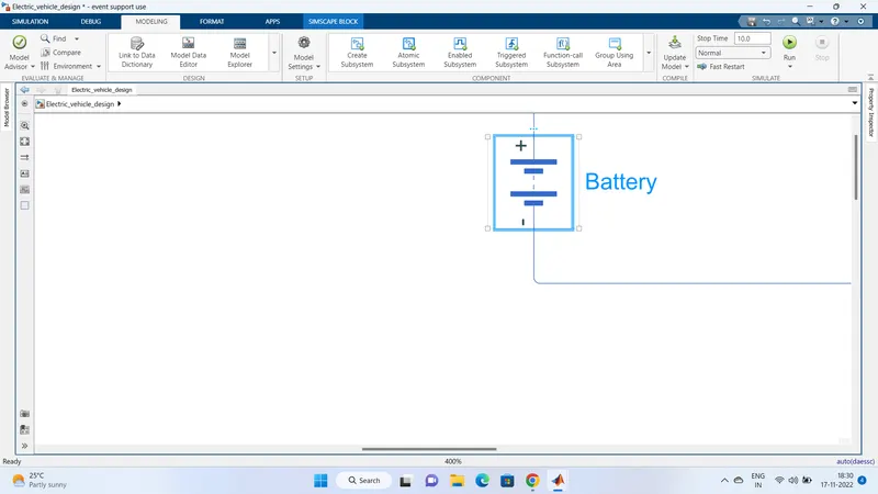
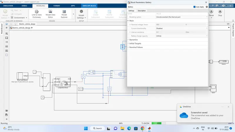
This block models a battery. If you select Infinite for the Battery charge capacity parameter, the block models the battery as a series of internal resistance and a constant voltage source. If you select Finite for the Battery charge capacity parameter, the block models the battery as a series of internal resistance plus a charge-dependent voltage source defined by:

V = Vnom*SOC/(1-beta*(1-SOC))

where SOC is the state of charge and Vnom is the nominal voltage. Coefficient beta is calculated to satisfy a user-defined data point.

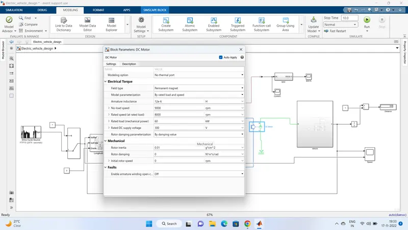
17) DC Motor:

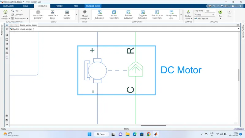
This block represents the electrical and torque characteristics of a DC motor. The block assumes that no electromagnetic energy is lost, and hence the back-emf and torque constants have the same numerical value when in SI units. Motor parameters can either be specified directly or derived from the no-load speed and stall torque. If no information is available on armature inductance, this parameter can be set to some small non-zero value. When a positive current flows from the electrical + to - ports, a positive torque acts from the mechanical C to R ports. Motor torque direction can be changed by altering the sign of the back-emf or torque constants. Here we are using a permanent magnet DC motor.

18) Mechanical Rotational reference:

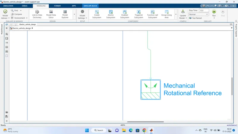
This block represents a mechanical rotational reference point, that is, a frame or a ground. Use it to connect mechanical rotational ports that are rigidly affixed to the frame (ground).

19) Scope:

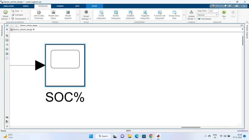
The scope is used to get the output of the system.

20) Integrator:

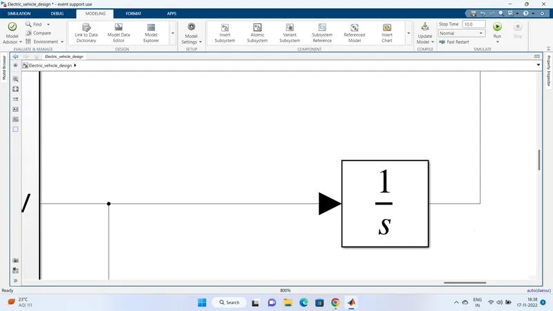
Continuous-time integration of the input signal.

21) Divide:

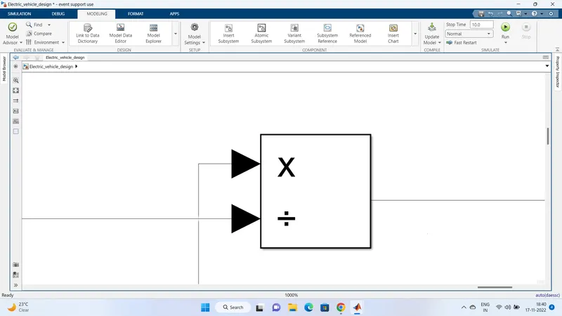
Multiply or divide inputs.

22) Rate Transition:

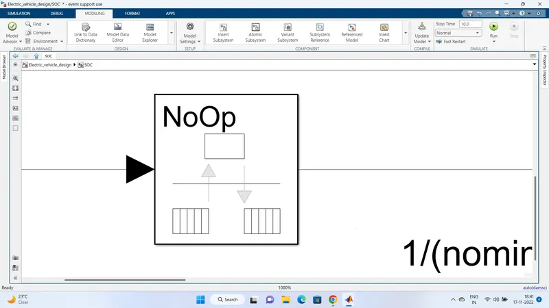
Handle data transfer between different rates and tasks.

23) Gain:

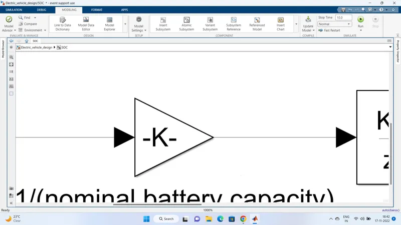
It Element-wise gain (y = K.*u).

24) Discrete-Time Integrator:

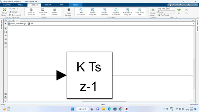
Discrete-time integration or accumulation of the input signal.

25) Sum:

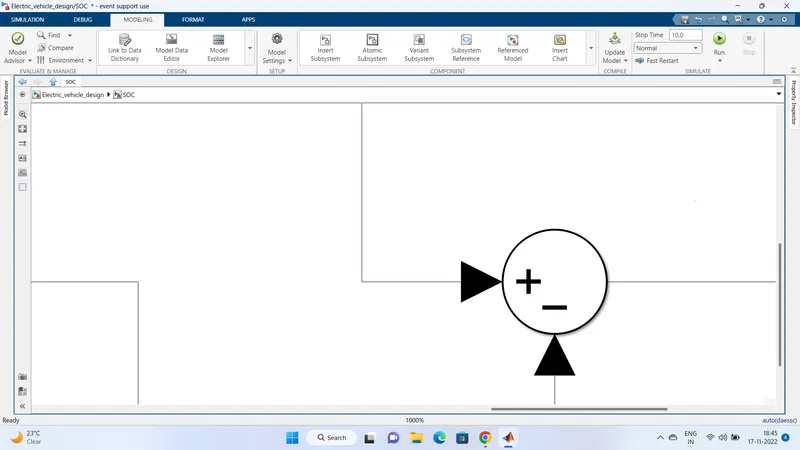
It is used to add or subtract.

26) Display:

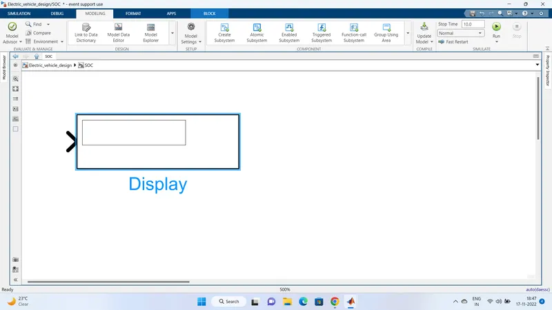
Display input or output values.

Model Construction and Explanation:

Vehicle subsystem:

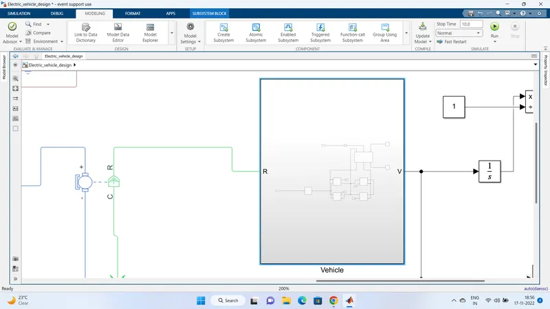
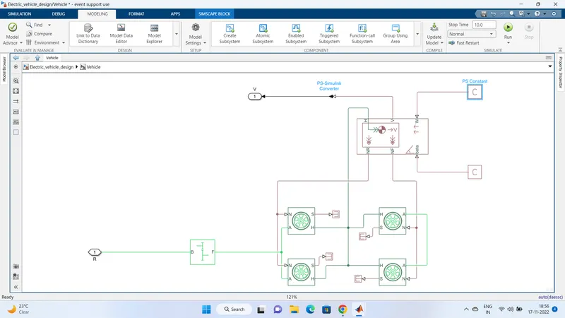
The vehicle subsystem blocks contain the tire arrangement 4 tires arranged as from wheels and rear wheels.The axle blocks are connected to the tire block next to each other to form as front axle and rear axle. Hub is also connected to hub.

A vehicle body block is present and the connections are made to the necessary connection ports of the tire.

For the simplification I had taken the simple gear.

The remaining ports are connected to constants or connection port.

SOC subsystem:

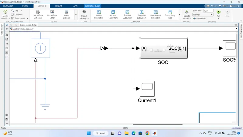
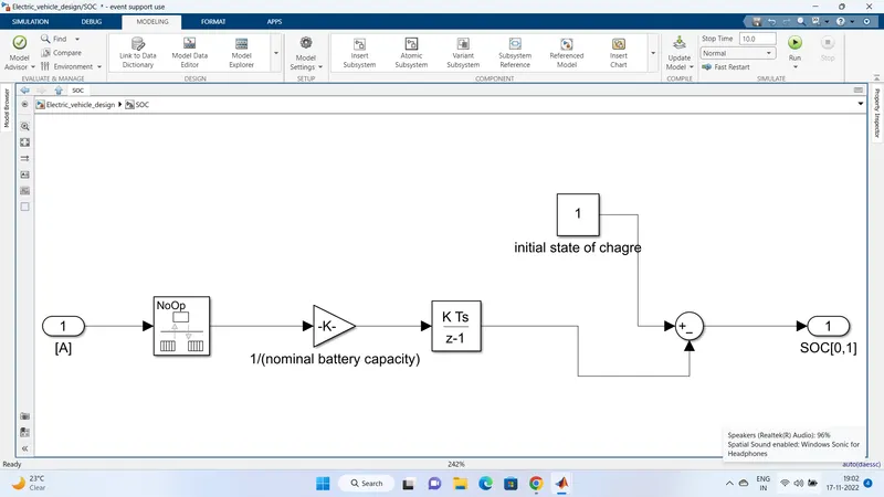
This is the subsystem to determine the state of charge of the system.

The rate transition block is connected to gain where gin is given 1/nominal battery capacity. It is further connected to the dicrete time integrator. The constant block is connected determining the state of charge. Here state of charge is full 1 as 100%.

Electric Vehicle Model:

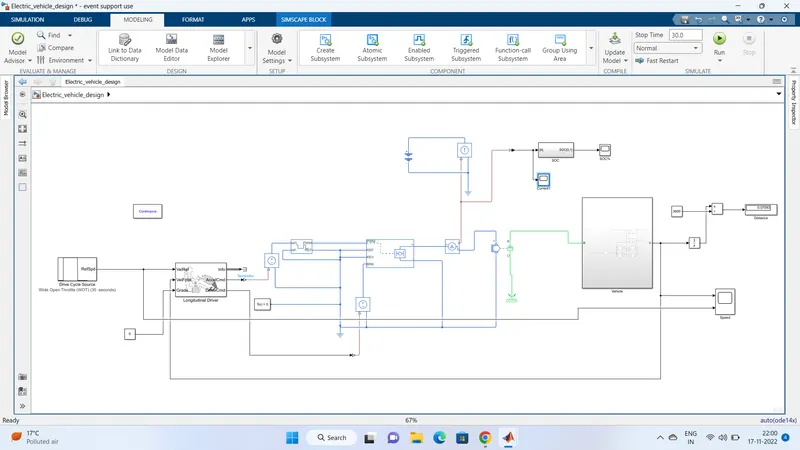
This the electric vehicle model designed and the model is also attached in slx format.

The parameters set are:

Vehicle body parameters

Tire parameters:

Controlled PWM Voltage:

DC motor parameters:

Drive cycle WOT:

Battery parameters:

Results:

I selected the drive cycle as wide open throttle and run the model for 30 seconds.

Solver settings are fixed step and automatic solver selection.

Current Scope:

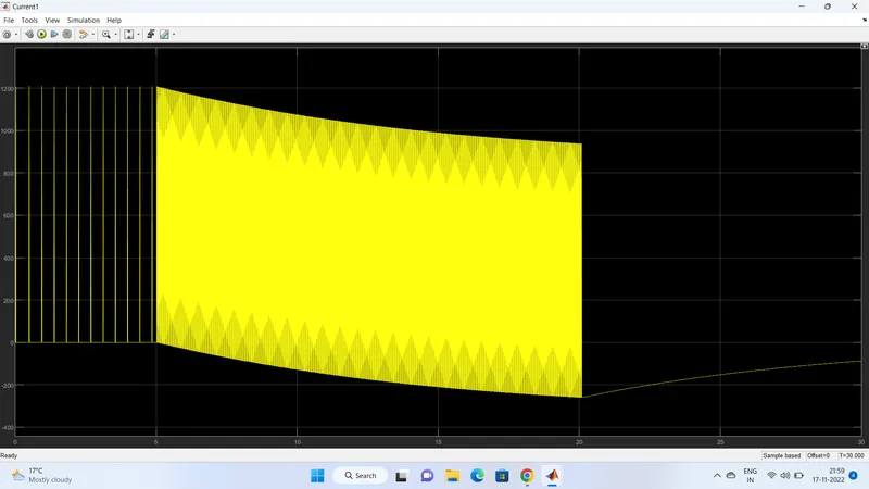
The current scope shows how the current flowing from the battery to the motor varies with the drive cycle time. As we can see, initially the current flowing through the circuit is 0A and this corresponds to the drive cycle commanding the vehicle to be at rest for this time period. At t = 5 seconds, when the vehicle is commanded to accelerate, the current instantaneously increases to a maximum current of 235.8A. This maximum current is achieved because at t = 5 seconds, the vehicle accelerates at maximum power under the WOT condition and so this will demand a high current from the battery. From t = 5 seconds to t = 17.5 seconds, the current decreases gradually to 134.3A. The current must have decreased over time because as the vehicle was accelerating, it required lesser current from the battery to continue accelerating. The highest current is always required when accelerating from rest due to the inertia of the vehicle. But once the vehicle is already in motion, it requires significantly lesser energy to continue accelerating. From t = 17.5 seconds to t = 20 seconds, the current flowing from the battery decreases more rapidly to 85.6A. This is because, at this time, the acceleration of the vehicle began to level off meaning that the increase in speed in those 2.5 seconds was lesser than the increase from t = 5 seconds to t = 17.5 seconds. 

After t = 20 seconds, the vehicle decelerates, causing the current to drop instantaneously to the negative axis to a value of -107.4A. There is now a negative current flowing due to regenerative braking. When the vehicle decelerates, the throttle is no longer applied and so the kinetic energy from the motion is converted to electrical energy fed back to the battery of the EV. This reverse flow of current is what causes the negative current measurement. From t = 20 seconds, the deceleration continues, however, the current flowing through the battery decreases in magnitude. This is because, at t = 20 seconds, the vehicle had reached its top speed and hence its maximum kinetic energy. So, at that point, there was more kinetic energy that could be converted to electrical energy for regenerative braking. However, as the vehicle decelerates, there was lesser energy available for regenerative braking causing the magnitude of the current to decrease. The polarity of the current hence moves towards the positive direction because regenerative braking happens lesser and lesser until the vehicle comes to rest. At t = 30 seconds, the vehicle is still decelerating and finished with a current measurement of -27.9A showing that regenerative braking is still occurring. 

Speed Scope:

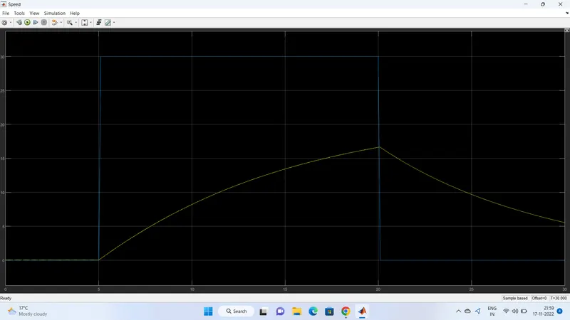
From this scope, we can see 2 signals. The blue signal represents the reference signal which originates from the drive cycle data whereas the yellow signal shows the actual velocity of the vehicle. The WOT drive cycle had been customized so that the vehicle begins acceleration under the WOT condition (i.e.. full power) at t = 5 seconds. This is supposed to be maintained till t = 20 seconds when the vehicle is supposed to begin deceleration. From t = 20 seconds to t = 30 seconds, the vehicle speed is back to 0m/s i.e. rest. Because this is a reference signal, all the commands are instantaneous. This is why the increase and decrease in speed are very sudden within a fraction of a second. However, this effect will not be observed in the actual velocity of the vehicle. This is because, in real-world conditions, there are more considerations to factor in which will not make it possible for a vehicle to accelerate and decelerate as instantaneously as the drive cycle commanded. In the real world, the effects of rolling resistance, drag, and road inclination make a difference because their presence would cause the vehicle's motion to deviate from the drive cycle commands. Other factors include the vehicle's inertia and the inertia of the transmission system. 

Observing the vehicle's actual velocity, as commanded, the vehicle begins at rest before accelerating under the WOT condition at t = 5 seconds. This acceleration is maintained till t = 20 seconds as the drive cycle commanded. At t= 20 seconds, the vehicle achieves a top speed of 26.8m/s.  After t = 20 seconds, the vehicle begins to decelerate gradually till t = 30 seconds where the vehicle finishes with a velocity of approximately 7m/s. As mentioned earlier, the actual velocity could not match the drive cycle commands perfectly and this is due to several factors which were discussed above. In my model, I have not modeled a road inclination but I have used a wind velocity of 5m/s. I compared the effect of this wind resistance on the top speed of the vehicle to when there was no wind resistance. The effect was very insignificant, only affecting the top speed by 0.5m/s. However, the vehicle velocity accelerated and decelerated as the drive cycle commanded. Obviously, the model is limited to the simulation time allotted. So if a longer simulation time is used, the vehicle may reach a higher top speed and may even decelerate back to rest. 

SOC scope:

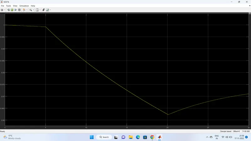
The SOC scope shows how the state of charge of the battery varies over the drive cycle time. The battery was modeled to begin with a SOC of 1 (100%) and so when the simulation begins, the SOC is at 1 until t = 5 seconds. This is because the drive cycle commands the vehicle to be at rest for that duration and so no discharge occurs from the battery. At t = 5 seconds, the vehicle is commanded to accelerate under the WOT condition and so the SOC of the battery decreases. Because the vehicle is accelerating at full power, the SOC falls from 1 but the rate of discharge decreases over the acceleration period eventually settling at a minimum SOC of 0.9914 at t = 20 seconds. This corresponds to the current flow from the battery because as the vehicle accelerates, lesser energy is demanded to increase the speed. As mentioned before, the greatest discharge occurs when the greatest current flows from the battery and this is during the initial acceleration period. As the vehicle speed increases, the acceleration decreases causing the current and hence the rate of discharge to decrease but in a mild fashion. At t= 20 seconds, the vehicle is commanded to decelerate and so the vehicle velocity decreases. This results in regenerative braking to occur which causes a negative flow of current back to the battery. Because this effect charges the battery, the SOC of the battery increases during the deceleration period. The SOC increases very gently from 0.9914 to 0.9935 and this is because the gets charged by the regenerative braking effect. The negative flow of current corresponds to the increase in the SOC of the battery. Since the vehicle is commanded to decelerate until t = 30 seconds, the vehicle speed decreases but does not reach 0m/s, so the vehicle is under regenerative braking for the entire period after t = 20 seconds.

Conclusion:

The total distance traveled is 0.07083 at a wide open throttle drive cycle.