Final Project: Design of an Electric Vehicle

AIM:

To create an Electric Vehicle Model using Simulink and Matlab.

THEORY:

An electric vehicle (EV) is a vehicle that uses one or more electric motors or traction motors for propulsion. An electric vehicle may be powered through a collector system by electricity from off-vehicle sources, or may be self-contained with a battery, solar panels, fuel cells or an electric generator to convert fuel to electricity. EVs include, but are not limited to, road and rail vehicles, surface and underwater vessels, electric aircraft and electric spacecraft.

EVs first came into existence in the mid-19th century, when electricity was among the preferred methods for motor vehicle propulsion, providing a level of comfort and ease of operation that could not be achieved by the gasoline cars of the time. Modern internal combustion engines have been the dominant propulsion method for motor vehicles for almost 100 years, but electric power has remained commonplace in other vehicle types, such as trains and smaller vehicles of all types.

Commonly, the term EV is used to refer to an electric car. In the 21st century, EVs have seen a resurgence due to technological developments, and an increased focus on renewable energy and the potential reduction of transportation's impact on climate change and other environmental issues. Project Drawdown describes electric vehicles as one of the 100 best contemporary solutions for addressing climate change.

Government incentives to increase adoption were first introduced in the late-2000s, including in the United States and the European Union, leading to a growing market for the vehicles in the 2010s. And increasing consumer interest and awareness and structural incentives, such as those being built into the green recovery from the COVID-19 pandemic, is expected to greatly increase the electric vehicle market. A pre-COVID 2019 analysis, projected that Electric vehicles are expected to increase from 2% of global share in 2016 to 22% in 2030. Much of this market growth is expected in markets like North America and Europe; a 2020 literature review, suggested that growth in use of electric vehicles, especially electric personal vehicles, currently appears economically unlikely in developing economies.

FIGURE.1

GOVERNING CHART:

The following flowing chart represents the working of electric vehicle and we used this flowchart to model our Electric Vehicle.

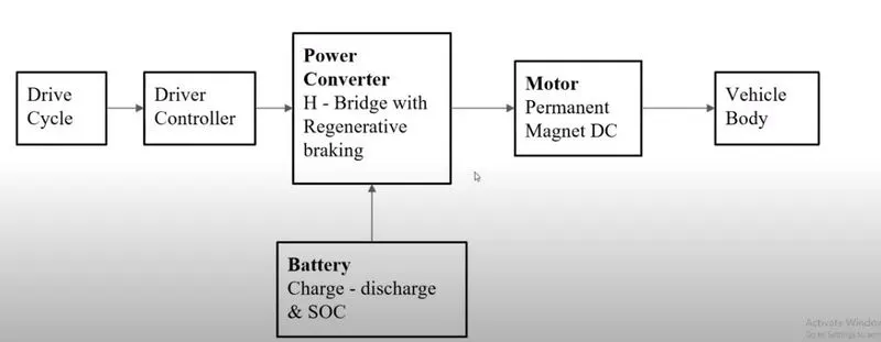
FIGURE.2

OBJECTIVES:

1. To make a simple electric vehicle model that uses DC motor and battery using Simulink.
2. To observe system level configuration and Model parameters.

SOLUTION:

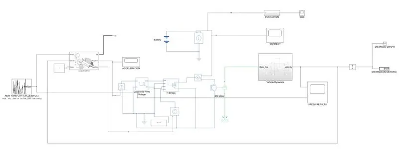
FIGURE.3

The above figure shows the model of an Electric Vehicle that we have made using Matlab and Simulink. All the speed units in this model are in Meter/Seconds.

The blocks used in this model are explained clearly as follows:

1. First, we have started modelling from the Wheels of the Vehicle, i.e.

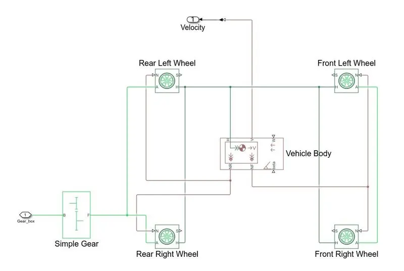
FIGURE.4

2. Here we can observe that we have used ‘Tire (Magic Formula) Block’, ‘Simple Gear Block’ and ‘Simple Gear Block’ to create the base for our model.
3. Firstly, we have used Tire Block and created four tires of the vehicle and named them as front and rear wheels. Here when we double click on the tire block, we get the following pop up box.

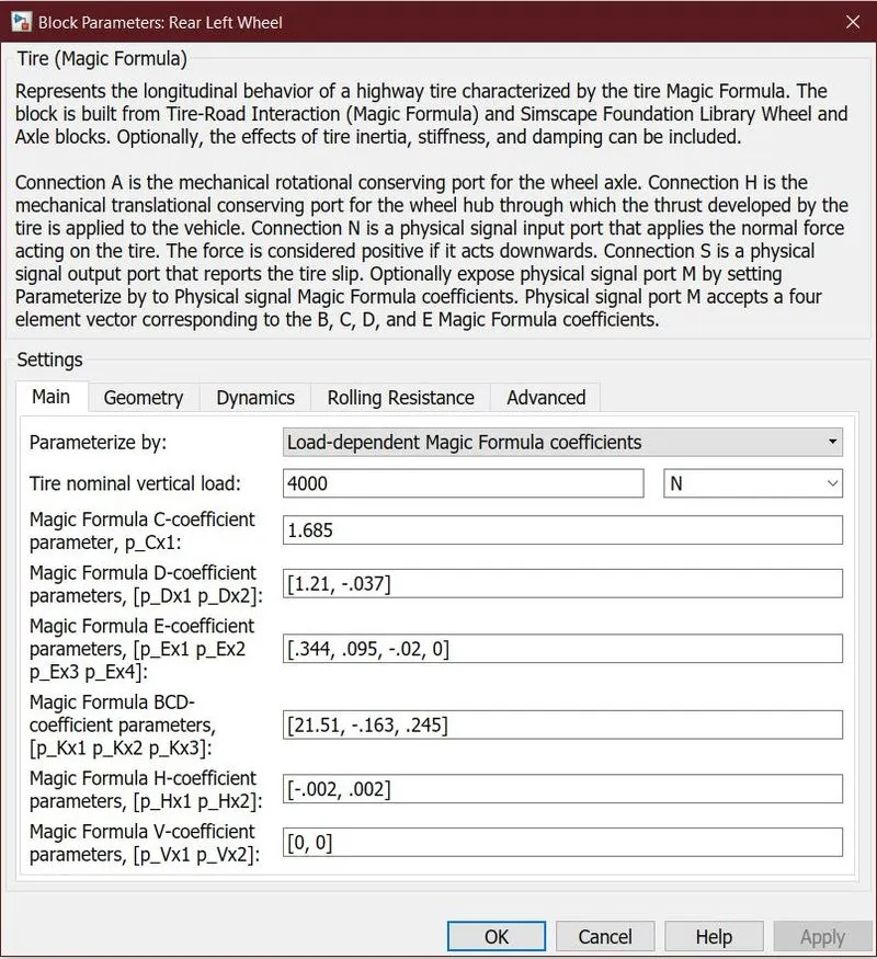
FIGURE.5

4. Here we can observe that there are various parameters, where we can edit according to our requirement. Here we have used default values for every Tire Block.
5. Then all the ports of each tire are is connect with each other, i.e. port “A” represents Axle so rear wheels “A” ports are connected with each other representing that they are on same single axle. Similarly, front wheels are also connected to same axle.
6. Then, the “H” port represents the hub so all wheels are connected to hub, i.e. all “H” ports are connected with each other.
7. Then, “N” and “S” represents the normal force and slip of the tire respectively. So, normal force on the rear wheels same, so “N” port of both rear wheel blocks is connected with each other and similarly for the front wheels normal force. Slip “S” port represents the slip occurring in the wheel. This port can be connected or left as it is. Its just gives the value of slip.
8. Then we have a used a “Vehicle Body Block”, where it represents the vehicle dynamics. If we double click on the this block, we get the following pop up box.

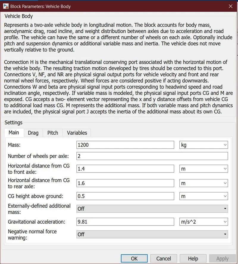
FIGURE.6

9. Here we can observe that there are various parameters which can be changed according to our requirement. In our model we have used the default values of this block.
10. Here ports “NR” and “NF” represent the normal force on rear tires and front tires respectively. So, the “N” ports of rear and front tires are connected with “NR” and “NF” ports according.
11. Now ports “H” represents the hub connection from the wheels, so as earlier we connected all the tires to hub. this connection is connected to “H” port of vehicle body.
12. Then port “W” and “Beta” represents the wind speed and road inclination angle which can be entered as input. In the above model we have not assigned any values as we have just modelled simple electric vehicle with simple calculation assuming its running on flat road.
13. The final port “V” represents the velocity output from the vehicle. So, this is connected to the output port. Then since the power from motor has to transmit to the wheels, we have used a transmission block i.e. “Simple Gear Block”. This block is connected to rear wheel axle since we have considered rear wheel drive.
14. Now all this setup together the made as subsystem where input of this system is the power given to the simple gear block and output is the velocity of the vehicle.
15. This subsystem is named as vehicle dynamics and then we have moved for selecting appropriate motor.
16. We have taken a simple “DC Motor Block” to represent a DC motor. When we double click on this block we get the following the pop-up box.

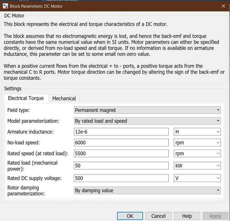
FIGURE.7

17. In the above parameters we have changed some of the parameters like the rated dc supply voltage of the motor, rated load, no-load speed, rated speed according our needs. These parameters can be changes according to the model needs later also.
18. Then, in the motor block 4 ports i.e. ‘-’, ‘+’, “C” and “R” ports are there, in this ‘-’ and ‘+’ port are the motor terminals where the power supply is connected and the positive torque of is from port “C” to “R”, so here port “C” is considered as fixed end of motor so its connected to ‘Mechanical Rotational Reference Block’.
19. Other port i.e. “R” is connected to the Vehicle Dynamic subsystem input, i.e. to simple gear block.
20. Then a controller is need to control the motor according to the needs, we need a controller block, for this we have used a “H Bridge Block”.
21. This block helps in controlling the drive of the motor. In this block the output voltage i.e. “-” and “+” port of this block is connected to the “-” and “+” of the DC motor block, which is nothing but input voltage for DC motor.
22. Then the PWM port is nothing but the PWM signal input port, here we can give a PWM input to this port. Then the REF and REV ports are grounded since we don’t need any reverse operation the motor using electric reference block. BRK port is connected to a constant voltage block which helps in doing regenerative braking.
23. When we double click on the “H Bridge Block” we get the following pop up box.

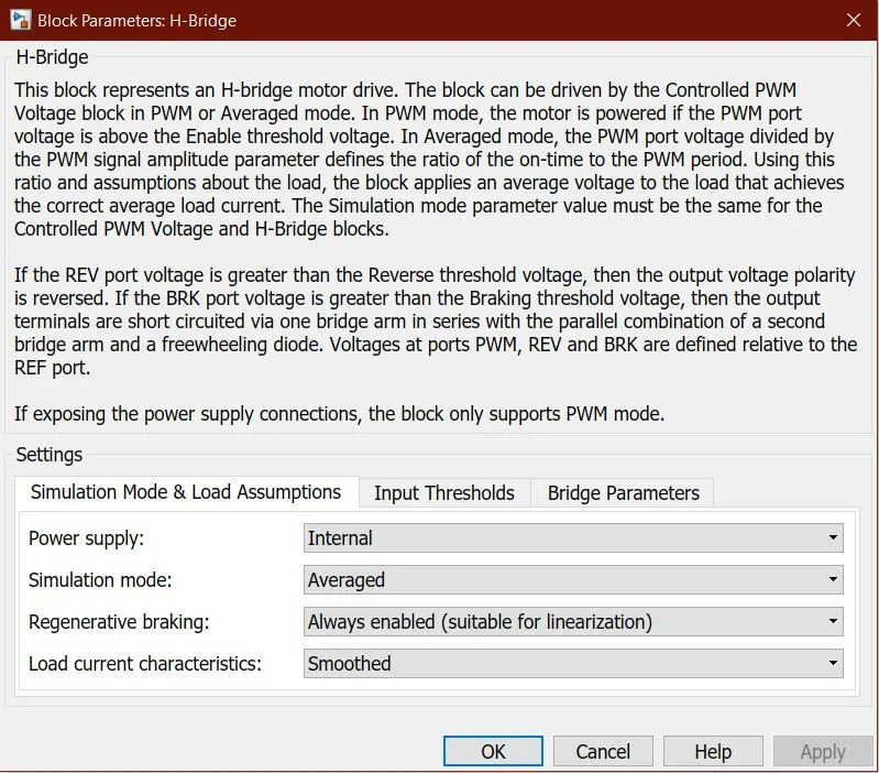
FIGURE.8

24. In the above parameters we have used same as defaults but we have changed the output voltage in the bridge parameters to same as the motor rated voltage.
25. Then to give PWM signals to the “H Bridge Block” we have used a “Controlled PWM Voltage” block. This block helps in creating the PWM Signals which are generated according to the variable voltages.
26. When we double click on this block we get the following pop up box.

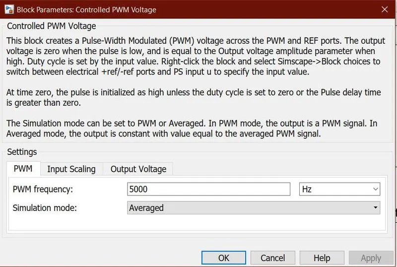
FIGURE.9

27. Here in the above parameters we have changed the frequency of the PWM signals thus increasing the duty cycle and simulation mode we have kept has Averaged so that when we run the model it takes less time.
28. The “PWM” and “REF” port of this block is connected to the “PWM” and “REF” port is the “H Bridge Block”. The “ref-” port is grounded since we don’t need negative voltage. The “ref+” port is connected to the “Controlled Voltage Block” so that input voltage is same always.
29. Then this block is connected to the “Longitudinal Driver Block” which is nothing but it represents the signal given by driver driving the car.
30. In this block the “VelRef” port is connected to a drive cycle and this drive cycle is continuously compared with the “VelFdbl” port where the vehicle speed is given as feedback. Whenever the vehicle speed is more than the drive cycle speed then the block will output as deceleration i.e. the “DecelCmd” port which is connected to one port of the “Controlled Voltage Port”. If the speed of vehicle is less than the drive cycle speed then the block will give output as acceleration i.e. “AccelCmd” port which is connected to Scope block.
31. This “Longitudinal Driver Block” is connected to a standard Drive cycle using Drive cycle block.
32. For the power source we have used a battery source Block which is connected to a constant current block. when we double click on Battery Block we get the following box.

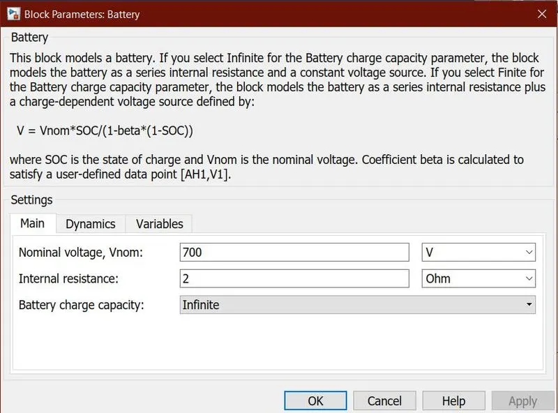
FIGURE.10

33. Here we have changed the voltage above to more than the rated voltage of the DC motor.
34. For calculating the SOC of the battery we have used another subsystem as shown below.
35. In this subsystem we can see that the current form battery is taken as input and connected to the “Rate Transition Block” where the data is transferred between different rates and tasks. Then “Gain Block” is used in order to update the signal coming from the rate transition block at constant gain. Then it is connected to the Discrete Time Integrator” block where discrete integration of the current signal is done with respect to time.
36. Thus, our EV model is completed and once we run the program we get the following results.

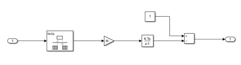
FIGURE.11

RESULTS:

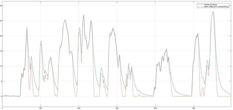
FIGURE.12

1. The above graph is the Speed Graph where the both drive cycle speed and vehicle speed are plotted. We can observe that the vehicle speed is near to the drive cycle speed which means our Electric vehicle meets the necessary speeds.

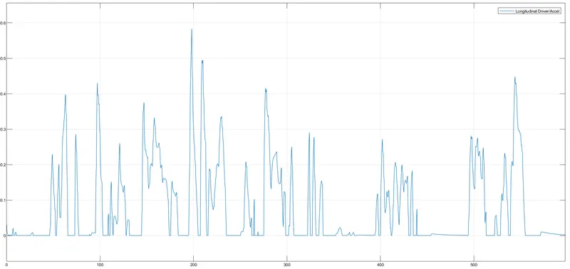
FIGURE.13

2. The above graph represents the acceleration applied by the driver during the drive, we can see that when speed has become less the acceleration also has decreased and when the speed has increased the acceleration has also increased.

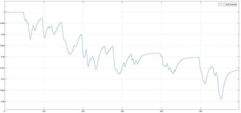
FIGURE.14

3. The above graph represents the SOC of the battery where the charge of the battery is less compared to the start when the drive has ended. This means that the power from battery has been used and at places it has be charged but charging is less than rate of discharging.

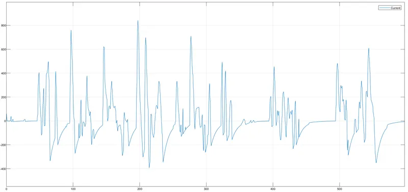
FIGURE.15

4. The above graph is the Current used by the vehicle. We can observe that current has been used where vehicle needed power to accelerate and at some places the vehicle has charged the battery i.e. when current is negative in the graph.

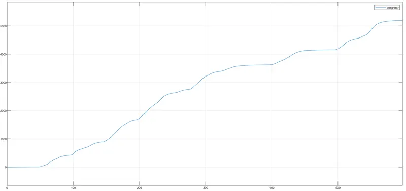
FIGURE.16

5. The above graph represents the distance graph where the distance is keeping on increasing as we have assumed that vehicle is moving only in positive direction.

CONCLUSIONS:

1. Thus, a simple Electric Model was modelled successfully.
2. Similar approach can be followed for modelling similar vehicle models in Matlab.
3. This model can be further improvised by increasing the complexity of the model for better results.
4. Further Extra features can be added to the Electric vehicle model.
5. Link for the above Simulink model:- https://drive.google.com/drive/folders/1iC9Ipdco7A3weAb6wBC7xUx9p97oExLh?usp=sharing