Week-4 Challenge WOT Condition Part-2

AIM:

To study HEV (Hybrid Electric Vehicle) and EV (Electric Vehicle) from Reference application projects in Simulink.

THEORY:

HEV (HYBRID ELECTRIC VEHICLE):

A hybrid electric vehicle (HEV) is a type of hybrid vehicle that combines a conventional internal combustion engine (ICE) system with an electric propulsion system (hybrid vehicle drivetrain). The presence of the electric powertrain is intended to achieve either better fuel economy than a conventional vehicle or better performance. There is a variety of HEV types and the degree to which each function as an electric vehicle (EV) also varies. The most common form of HEV is the hybrid electric car, although hybrid electric trucks (pickups and tractors) and buses also exist.

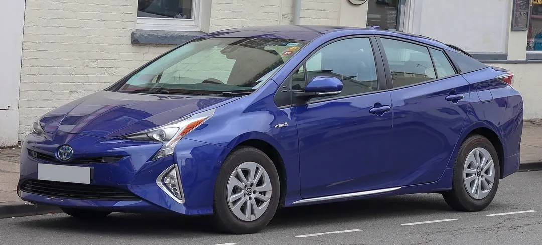
FIGURE.1: TOYOTA PRIUS

EV (ELECTRIC VEHICE):

An electric vehicle (EV), also called electrics is a vehicle that uses one or more electric motors or traction motors for propulsion. An electric vehicle may be powered through a collector system by electricity from off-vehicle sources, or may be self-contained with a battery, solar panels, fuel cells or an electric generator to convert fuel to electricity. EVs include, but are not limited to, road and rail vehicles, surface and underwater vessels, electric aircraft and electric spacecraft.

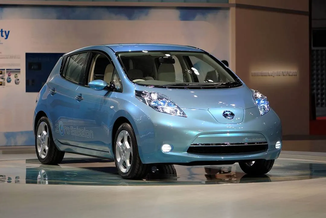
FIGURE.2: NISSAN LEAF

OBJECTIVES:

1. To discuss what is the difference between mapped and dynamic model of engine, motor and generator? To check how can we change model type?
2. To see how does the model calculate miles per gallon? Which factors are considered to model fuel flow?
3. To run the HEV Reference Application with WOT drive cycle and to change the grade and wind velocity in the environment block and comment on the results.
4. Keeping all other parameters same, compare the simulated results of hybrid and pure electric powertrains.

Link for HEV reference model: https://in.mathworks.com/help/autoblks/ug/explore-the-hybrid-electric-vehicle-multimode-reference-application.html

Link for EV reference model: https://in.mathworks.com/help/autoblks/ug/explore-the-electric-vehicle-reference-application.html

SOLUTION:

DIFFERENCE BETWEEN MAPPED AND DYNAMIC MODELS OF ENGINE, MOTOR AND GENERATOR

Mapped Motor: It is also known as static motor where the model runs based upon look up tables or some predefined input values. Simulation using this model is fast than the dynamic model.

Dynamic Motor: This model represents the real time working of the model. It represents the actual model of the equipment. It does not take any predefined values as input. It takes the real time values as inputs and gives the output continuously. Simulation using this model is slow compared to Mapped Motor model.

Mapped Generator: This is also similar like the mapped motor, where the input values for the generator block are predefined or it takes from the lookup tables. Here also simulation time is less when this model is used.

Dynamic Generator: This model also represents actual generator which work in a real time environment. Here the input values are not taken from look up tables, the output values are calculated continuously according to the changes in input values. Here also simulation time is more compared to mapped generator.

Mapped Engine: It is a steady-state model where all the input parameters like air mass flow, fuel flow, exhaust temperature, efficiency, and emission performance are taken from look tables where values are predefined. Simulation time here is less when this model is used.

Dynamic Engine: This model also represents the actual working of the engine in real time. The input values change every time so the output values from the model also changes continuously. Here also simulation takes more time to complete.

To change the model from dynamic to mapped,

1. In the reference application model where ever the mapped model is used, below that a dynamic model is also present and its connected out since the connection s are given to mapped models.
2. To use the dynamic model, first we have to comment out the mapped model and then connect all the inputs to the dynamic model.
3. Similar way is used to change from dynamic to mapped model.

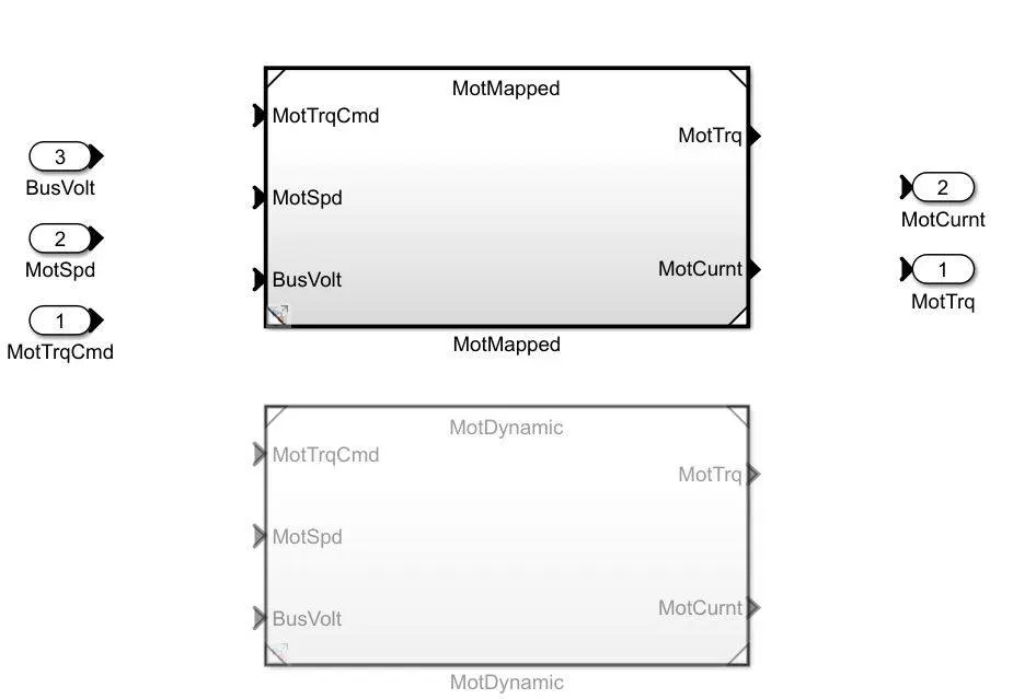
FIGURE.3

4. The above picture shows the two models where the dynamic model is commented out.

CALCULATING THE MILES PER GALLON

1. Usually to calculate miles per gallon, the automobile is first filled with fuel fully until its fuel tank is full. Then the distance travelled in odometer in noted and then the automobile is started and is used until all the fuel is consumed thus emptying the fuel tank.
2. Now again the distance travelled is noted down and the difference between both the readings of distance travelled is found out. Then this difference value is divided by the total fuel tank capacity of the automobile, thus the resulting value obtained is the average mileage of the automobile in miles per gallon
3. For example, if the vehicles initial odometer reading is 2000 miles and its fuel capacity is 10 gallons, after filling the fuel completely and starting the trip, at the end of trip i.e. when all the fuel is over, the reading on the odometer is 3000 miles then,

Difference in Distance `= 3000-2000 = 1000` miles

Fuel Tank Capacity `= 10` gallons

therefore, its mileage is `1000/10 = 100` miles per gallon

4. In the Simulink model, it also calculates the performance in the similar manner.

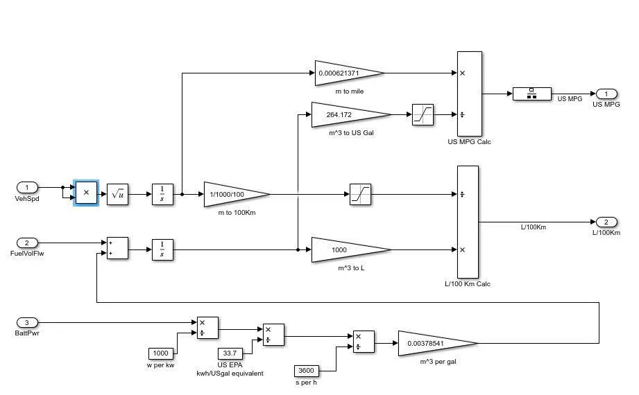
FIGURE.4

5. The above figure shows how the model calculates miles per gallon. Above model can be found in the ‘Visualization Block’ of the HEV model and in the ‘Visualization Block’ click on ‘Performance Calculation’ block then the above model will open.
6. In the above model we can observe that FACTORS that are needed as inputs to the model are Vehicle Speed, Fuel Volume Flow and Battery power. As these values changes the performance of the vehicle also changes.
7. Here first the velocity of the vehicle is converted into distance by integrating the velocity values and then distance is converted from meters to miles and km.
8. Then similarly battery power is converted into volume by multiplying and dividing by constant conversion values. Then the battery and fuel volume flow are added and integrated to get the total volume of fuel consumed. Now this volume is converted from cubic meter to gallons and litres.
9. Now the distance and volume of fuel id divide to get the performance results in miles per gallon and litres/100km.
10. Factors that are required to model fuel flow are battery power, conversions from watt to cubic meter per gallon.

TO RUN HEV REFFERENCE MODEL IN WOT DRIVE CYCLE:

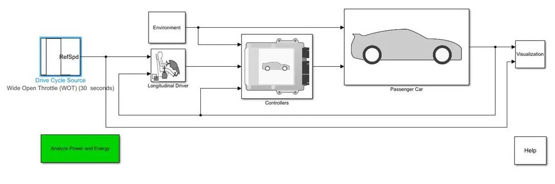
FIGURE.5

1. To change the drive cycle, click on the ‘Drive Cycle Source’ block and from the drop down, select WOT option.
2. Now run the model to observe the results.

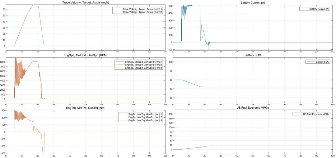
FIGURE.6

3. We will the above results once the simulation has ended. In the first graph we can see the difference between drive cycle and actual velocity change. To attain maximum speed, it takes nearly 18 seconds and to reach zero velocity from maximum velocity it takes nearly 5 seconds. So, to reach top speed and again come back to rest it takes total of 23 seconds. So, the actual time varies from the drive cycle time.
4. In the second graph we can observe that while achieving the top speed, the speed of motor is varying continuously and once achieved the speed of motor is constant and then the speed reduced continuously to zero. High speed of motor is observed when the vehicle is reaching maximum speed.
5. In the third graph we can observe that the motor is giving high torque to achieve the top speed and then slowly is its reducing. Once it reaches the top speed then the motor torque slowly reduces and reaches zero. From here it goes negative because the motor is rotating due to vehicle speed thus the torque produced is due to vehicle, not due to motor so, its negative.
6. In the fourth graph we can see that the current consumed by motor is high when vehicle is achieving top speed and is constant until the speed is maximum and then as the vehicle speed decreases the current also decreases and a point it goes to negative which means that it charged due to regenerative braking and then again becomes zero.
7. In the fifth and sixth graph we can observe that the state of charge (SOC) has decreased as to achieve top speed some battery charge is used. And for fuel economy graph we can see economy is less initially as more fuel is needed to achieve top speed and then slowly it increases as the need of fuel decreases.

TO COMPARE THE RESULTS OF HYBRID AND PURE ELECTRIC VEHICLE:

1. By clicking the above link of EV reference model following model will open which will similar to that of HEV reference model, nut inside EV model there will no Engine model or block. The drive cycle is changed like the previous model to WOT drive cycle.

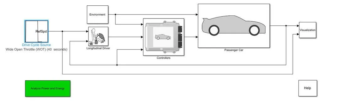
FIGURE.7

2. Now when we run the model, we get the following results.

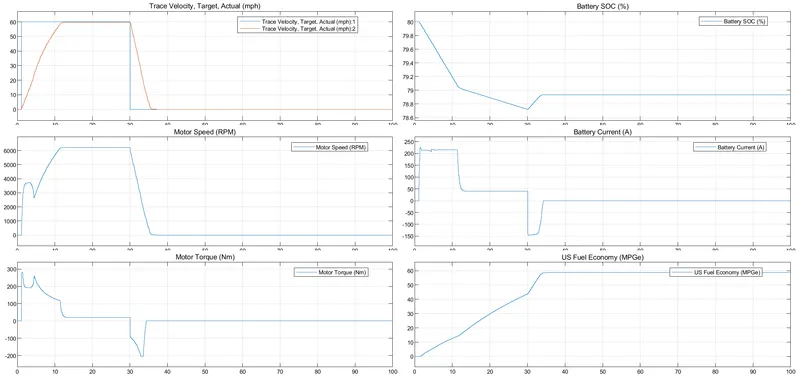
FIGURE.8

3. Here in the above figure, in the first graph we can see the top speed is achieved nearly at 14 seconds which very quick than the HEV model graph the time taken to come to zero velocity from top speed is nearly 5 seconds. So totally its takes 19 seconds to achieve top speed and come back to rest, which is quick than the HEV model.
4. In the second graph, we can observe that the graph is much smother than the HEV model. Thus, in electric vehicle the motor speed is smoother than the HEV motor speed.
5. In the third graph, here also the torque od motor is much smoother than HEV model an we can also observe that while the vehicle is decelerating, it is in regenerative braking mode, that’s why the torque is negative while deceleration.
6. In the fourth graph, the SOC of battery is decreases slowly like HEV model but here it decreases much more than the HEV model. Since in electric vehicle only battery is used so battery is consumed more thus while achieving top speed the SOC line in the graph falls down more than that of HEV model graph. Since regenerative braking is happening, which charges the battery so the curve has raised little bit at the end.
7. In the fifth graph, we can observe that the current consumed the EV is less than that of HEV as the mass of EV is less so less current to used compared to HEV. Here due to regenerative braking, more current is produced than that of HEV to charge the battery.
8. In the sixth graph, we can see that the fuel economy the vehicle is very high than that of HEV. Thus, concluding that EV is now fuel efficient than HEV.

CONCLUSIONS:

1. Thus, all the objectives were achieved successfully.
2. Similar kind of approach can be followed to study similar models in Simulink and Matlab.