Week-3 Challenge: ADVISOR Tool

AIM:

To perform simulation on various vehicle modules with different conditions using ADVISOR Tool.

THEORY:

ADVISOR, NREL’s ADvanced VehIcle SimulatOR, is a set of model, data, and script text files for use with Matlab and Simulink. It is designed for rapid analysis of the performance and fuel economy of conventional, electric, and hybrid vehicles. ADVISOR also provides a backbone for the detailed simulation and analysis of user defined drivetrain components, a starting point of verified vehicle data and algorithms from which to take full advantage of the modelling flexibility of Simulink and analytic power of MATLAB. The models in ADVISOR are mostly empirical, relying on drivetrain component input/output relationships measured in the laboratory, and quasi-static, using data collected in steady state (for example, constant torque and speed) tests and correcting them for transient effects such as the rotational inertia of drivetrain components.

ADVISOR was preliminarily written and used in November 1994. Since then, it has been modified as necessary to help manage the US DOE Hybrid Vehicle Propulsion System subcontracts. Only in January 1998 was a concerted development effort undertaken to clean up and document ADVISOR. Since then, over 4500 individuals have downloaded one or more versions of ADVISOR, including all of the OEMs and major suppliers. About 2/3 of the users are from industry and 1/3 from universities. A short list of major ADVISOR users includes DaimlerChrysler, Ford Motor Company, General Motors Corp, Delphi Automotive Systems, Visteon and hundreds of others.

FIGURE.1

OBJECTIVES:

1. To change the default value of cargo mass value to 500kg for Ev_defaults_in file in ADVISOR Tool, with keeping all other default conditions to find out whether the vehicle can travel 45km with FTP drive cycle.
2. For the same above case, now to change the battery condition and run the simulation.
3. To perform Gradeability test on PRIUS_Jpn_defaults_in file.

SIMULATION:

CHANGING THE CARGO MASS OF Ev_defaults_in FILE:

1. Firstly, when the ADVISOR tool opened, we have selected the units to be ‘metric’ and then from dropdown menu in ‘Load File’ bar.

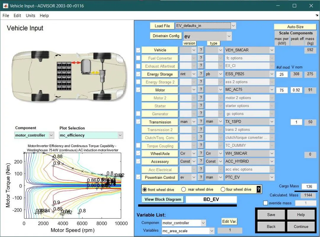
FIGURE.2

2. In the above figure we can observe that the default ‘Cargo Mass’ is 136 kg. now this value will be changed to 500 kg and the ‘Continue’ option is clicked.

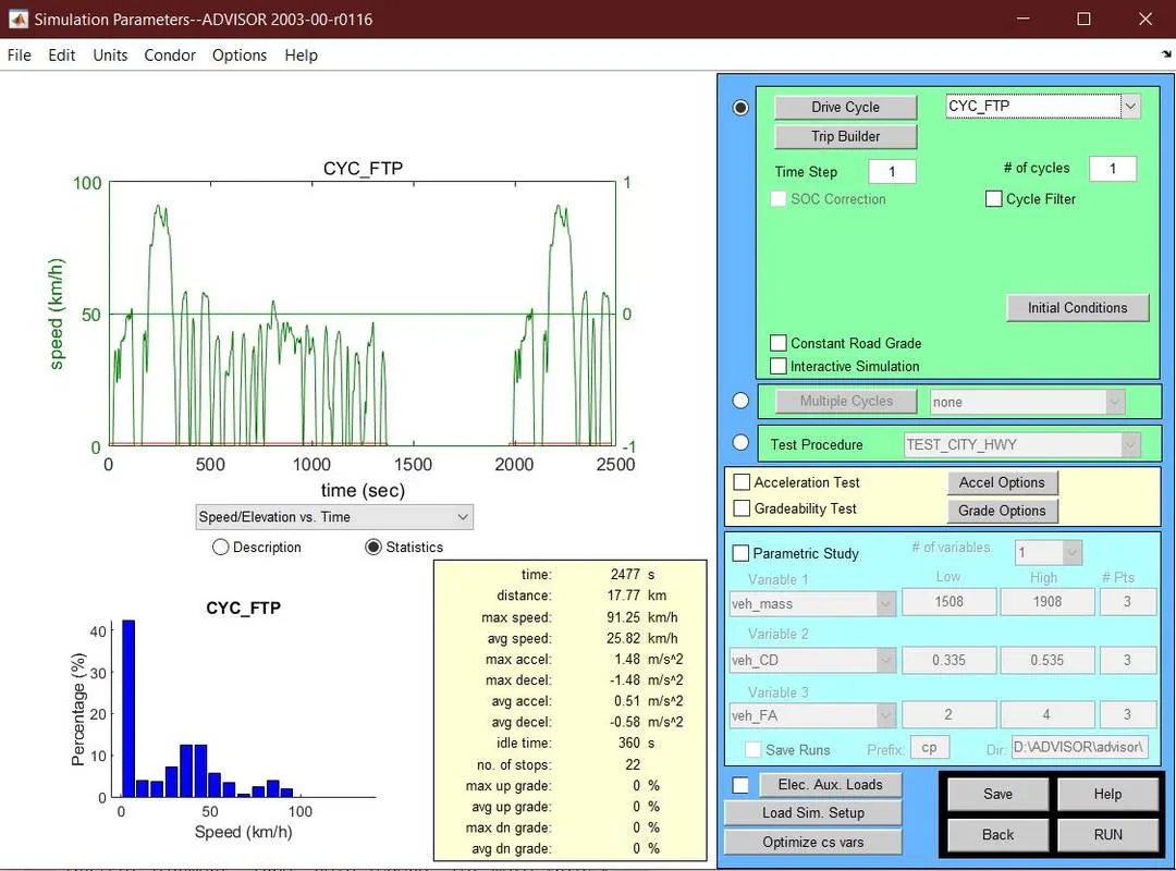
FIGURE.3

3. Once we click on the ‘Continue’ option we get a window like above figure. Here we can observe that by default in the ‘Drive Cycle’ bar ‘CYC_UDDS’ is selected. So, we have changed this to ‘CYC_FTP’ from the dropdown menu in ‘Drive Cycle’ bar.
4. Now click on the ‘RUN’ option to run the simulation.

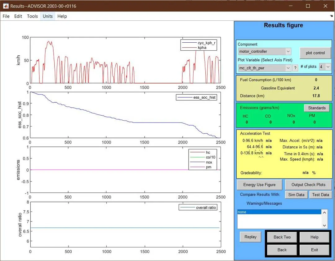
FIGURE.4

5. Once the simulation is finished, we will get the results as shown in the above image. Here we can see that in the results the distance travelled is less than 45 km, which means that if cargo load is 500 kg, the vehicle can cannot travel 45 km with the power it generates. It is nothing but the power source is not enough to carry a cargo load of 500 to travel 45 km.
6. Here distance depends on the type of ‘Driving Cycle’ and for how many cycles of the ‘Drive Cycle’ the simulation is run.
7. Here we have only simulated for one cycle of ‘FTP Drive Cycle’ so the distance covered in this cycle is only 17.8 km which is less than 45 km.

CHANGING THE BATTERY CONDITIONS:

1. Now here we can see that to change the battery conditions, we have changed the value greater than the default value in the ‘Energy Source’ option as shown in the below figure.

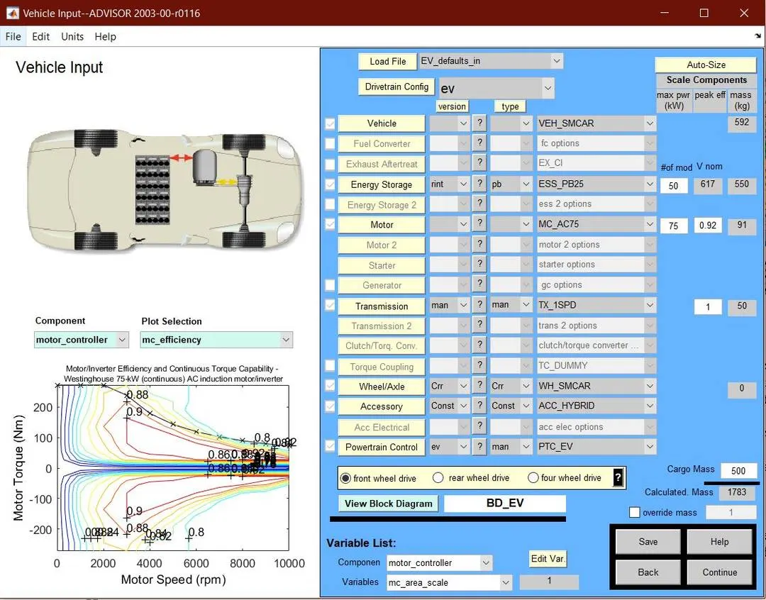
FIGURE.5

2. Keeping all the other parameters same except the ‘Energy Storage’, is changed to the value of 50 kW. Then click on ‘Continue’ option to proceed further.
3. In the next window we have kept all the parameters and their values unchanged a then clicked on ‘RUN’ option to run the simulation.

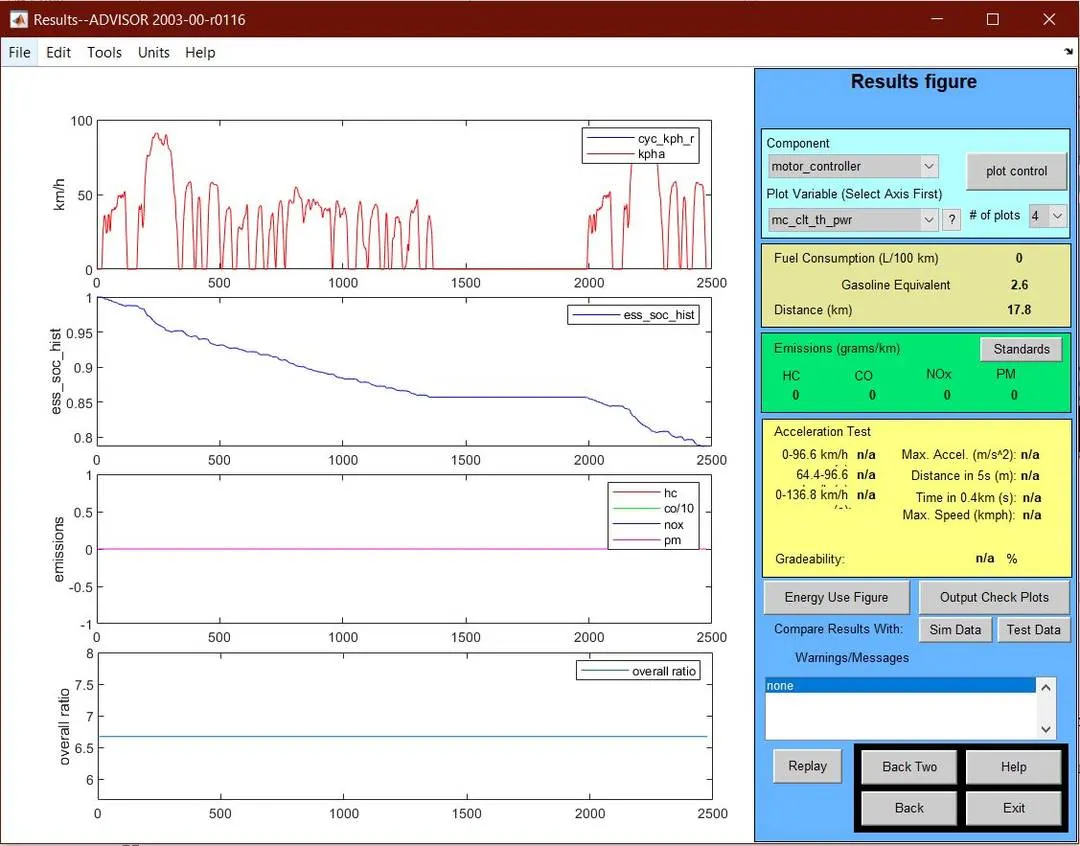
FIGURE.6

4. In the above picture we can see that there is no change in the value of distance since depends on number of cycles of the drive cycle. To observe the results related to battery, click on the option ‘Energy Use Figure’, this will show us the energy related observations.

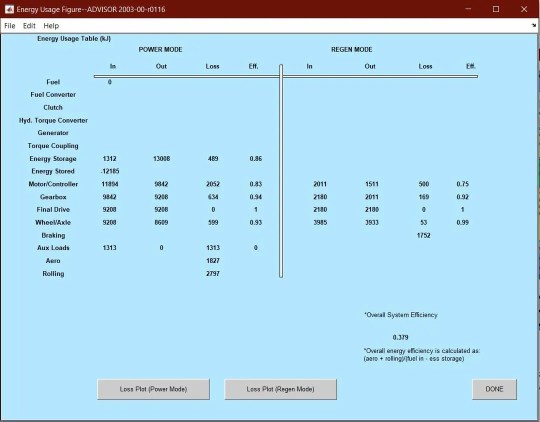
FIGURE.7

5. We will get window as shown in the above figure, in this we can observe that, in the ‘Energy Storage’ row we see the values that how much power is spent from the battery and how much power is given to the battery.
6. In the ‘Power Mode’ section, ‘In’ column refers to the amount of power given to the battery and ‘Out’ column refers to the amount of power spent from the battery, similarly we can also observer the efficiency and amount of losses in the battery also.
7. Now the same simulation is run with the value of ‘Energy Storage’ less than the previous simulation to compare the results observe the difference in both the simulations.

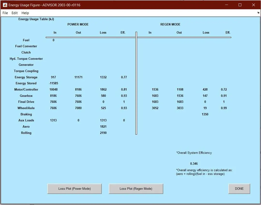
FIGURE.8

8. Above figure is the results of the simulation where the value of the ‘Energy Storage’ is less than the previous simulation ‘Energy Storage’ value.
9. Here the values in the ‘Energy Storage’ row are less than the previous simulation as the value of the ‘Energy Storage’ is less. So, as the value of ‘Energy Storage’ is decreased we will get less power to spent for the vehicle. The over all efficiency is also changing proportionally to the ‘Energy Storage’ value.
10. Thus, change in battery value that is change in ‘Energy Storage’ values, changes the value of power output from the vehicle power source.

PERFORMIMG GREADEABILITY TEST ON PRIUS_JPN_DEFAULT_IN FILE:

1. To perform gradeability test on the ‘PRIUS_Jpn_defaults_in’ file, first from the dropdown menu of ‘Load File’ bar we have selected PRIUS_Jpn_defaults_in file.
2. Then keeping all the default values of the parameters, we have clicked on the ‘Continue’ option.

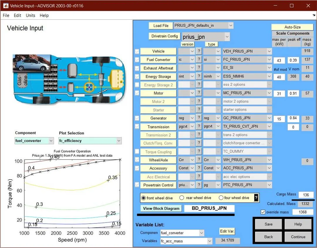
FIGURE.9

3. Then, in the next window we can observe that there are two options ‘Acceleration Test’ and ‘Gradeability Test’, since we need only the gradeability test, we have ticked on ‘Gradeability Test’.

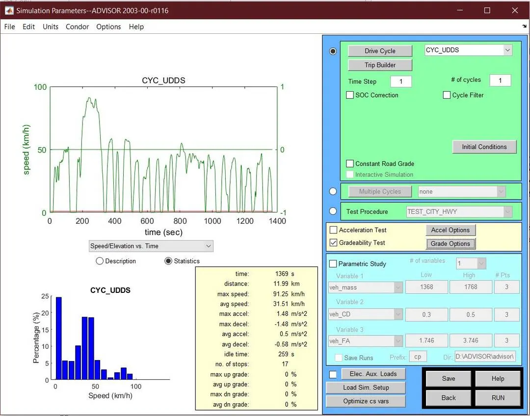
FIGURE.10

4. We can also observe that there is an option adjacent to ‘Gradeability Test’ named as ‘Grade Option’. By clicking on this we get the following options.

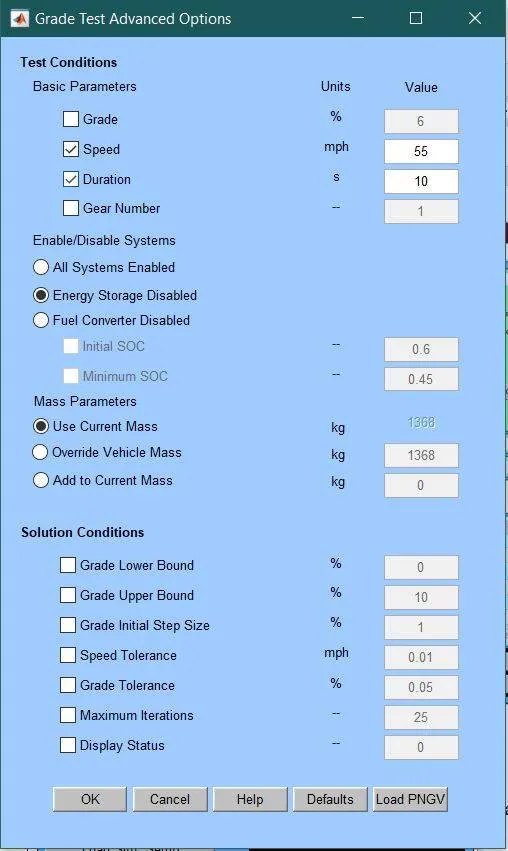
FIGURE.11

5. Here we can observe the test conditions, here we can adjust the parameters according to our requirements and then run the test. Here we can set the gradeability of the vehicle, speed of the vehicle when that particular gradeability is there and the till how much time that gradeability is present.
6. By keeping the default values we have the run the simulation and got following results.

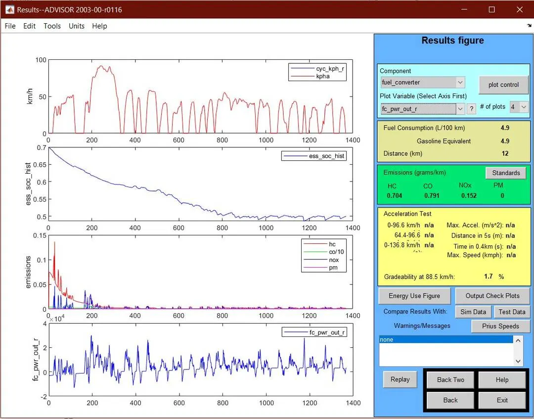
FIGURE.12

7. Above figure shows the results of the simulation, where we can see that the Gradeability at 88.5 kmph speed is 1.7%. This tells that only 1.7% gradeability can only be achieved by the vehicle at the speed of 88.5 kmph.
8. Since our grade value is set to 6% by default in the ‘Grade Option’ menu but the we got only 1.7%, which means that we have got lesser value than our desired value.
9. Now let us run a simulation by changing the values in the ‘Grade Option’ menu and then observe the results.

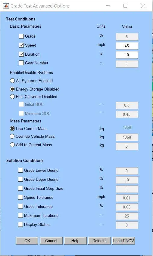
FIGURE.13

10. Above results are obtained by changing the speed value in ‘Grade Option’ menu. Now we can observe that the maximum possible gradeability is more than the previous simulation that is 2.2% but the maximum speed has decreased.
11. Now let us run the simulation further by changing the values in ‘Grade Option’ menu and compare the results with previous simulation results.

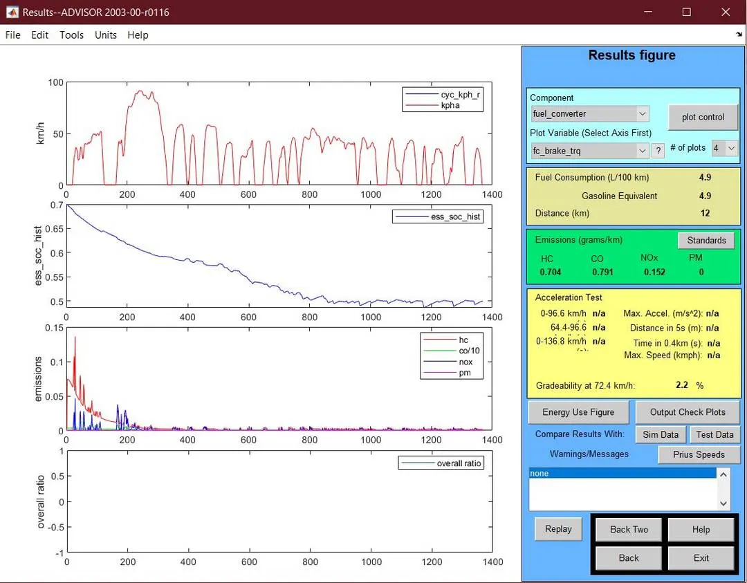
FIGURE.14

12. In the above results we can see that as further we decreased the speed in the ‘Grade Options’ the gradeability of the vehicle has increased.
13. The reason for this change is, when a vehicle is travelling at high speed it requires more power and adding to this if it needs to climb a slope at high speed further more power is required. Here in this study case our power amount is fixed, if the gradeability and speed requirement is high, we cannot get desired results as power is not sufficient.
14. Therefore, the if the speed is at optimum value (usually 30 kmph to 60 kmph) a decent gradeability can be achieved and if we need further more gradeability we have to increase the power output of engine and battery.
15. So, in this case at 48.3 kmph we get the maximum possible gradeability.

Speeds (in kmph)	Gradeability (%)
160.9	n/a
144.8	0.3
128.7	0.3
120.7	0.7
88.5	1.7
72.4	2.2
48.3	2.5
40.2

TABLE

16. The above table show gradeability of vehicle at different speeds. Here we can at higher speed there no gradeability achieved with the total available power and similarly at lower speed also there is no gradeability achieved with the total available power as at lower speed more torque is required.

CONCLUSION:

1. Thus, all the objectives were achieved successfully.
2. Similar kind of approach can be used to study similar kind of simulations.