Simulink- WEEK_1

AIM:

To plot a function using basic Simulink blocks and to run and study a Simulink example ‘Suspension System Comparison’.

SUSPENSION:

Suspension is the system of tires, tire air, springs, shock absorbers and linkages that connects a vehicle to its wheels and allows relative motion between the two. Suspension systems must support both road holding/handling and ride quality, which are at odds with each other. The tuning of suspensions involves finding the right compromise. It is important for the suspension to keep the road wheel in contact with the road surface as much as possible, because all the road or ground forces acting on the vehicle do so through the contact patches of the tires. The suspension also protects the vehicle itself and any cargo or luggage from damage and wear. The design of front and rear suspension of a car may be different.

GOVERNING EQUATIONS:

The function to be plotted is given as:

`y(x)=(x-1)*(x-3)^2*(x-9)^2`

OBJECTIVES:

1. To plot above function using Simulink blocks.
2. To Study a Simulink Example and find answers for following question:-

1. What is the objective of the simulation? What are the similarities and differences between the three systems understudy?
2. What are your observations from the results?
3. How the oscillating velocity source is created?

MODELS:

FUNCTION MODEL:

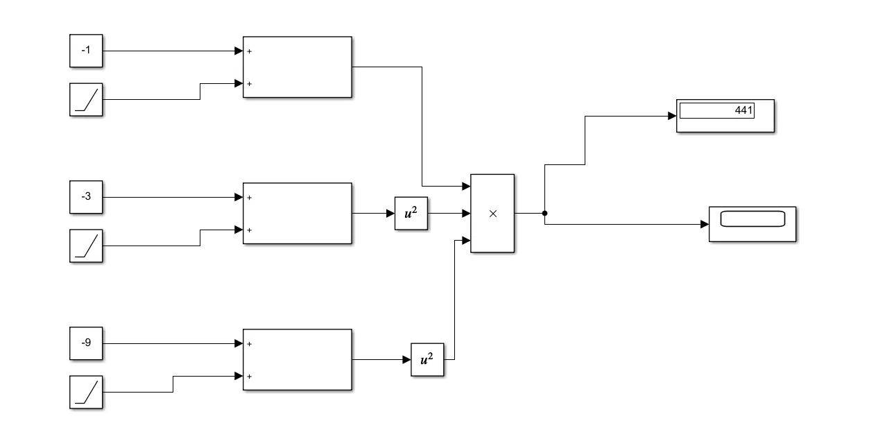
FIGURE.1

EXPLANATION

1. In the above Simulink model, blocks that are used are sum block, constant block, ramp block, math function block, product block, display block and a scope block.
2. First we have divided the function into three parts i.e. first part is ‘(x-1)’ , second part is ‘(x-3)^2’ , third part is ‘(x-9)^2’. Then we can multiply all three parts to get the final answer of the function.
3. Now to achieve three parts, we have taken SUM BLOCK from the ‘Library Browser’ , since we have three parts we have taken three SUM BLOCKS. In the SUM BLOCK we can observe that the inputs are denoted with symbol ‘+’ which means the inputs will be added and the output will be their sum. U can modify these inputs by double clicking in the SUM BLOCK. This block can also be used for subtracting by changing the inputs of the SUM BLOCK.
4. Here in the above model, without changing the inputs we have used this block. Now to one of the input of SUM BLOCK is connected by a CONSTANT BLOCK. This block helps use to give any constant value as inputs. Since in first part of equation constant value is ‘-1’ so this value is given for the CONSTANT BLOCK. This constant is one input for the SUM BLOCK.
5. Now in the first part of the function, variable is ‘x’ so to represent this RAMP BLOCK is used. RAMP BLOCK is a signal which changes continuously w.r.t time i.e. it acts like a variable. If we double click on the RAMP BLOCK we can see a row where it is defined as ‘Slope’ , this values is the increment value for the RAMP BLOCK, i.e. the value in RAMP BLOCK in increased by the value of slope for each second of time. By default value of slope is ‘1’, so in our model RAMP BLOCK will increase by 1 for every second. Initial value and intial time for starting thr RAMP BLOCK is set to ‘0’ by default.
6. Now this RAMP BLOCK is assigned as second input for the SUM BLOCK. So by assigning the inputs to the SUM BLOCK the output is given as (x-1), which is first part of our function.
7. Similarly for second and third part of the function same approach is used to find (x-3) and (x-9). Now to square these terms, the output of SUM BLOCK of these two terms is given input to a MATH FUNCTION BLOCK and by double clicking it we have selected squaring math function in that block.
8. Now output of first SUM BLOCK, first MATH FUNCTION BLOCK and second MATH FUNCTION BLOCK represent (x-1), (x-3)^2, (x-9)^2 respectively. As per the equation we have multiply all these terms to get the final value of the given function.
9. So these outputs are given as inputs to a PRODUCT BLOCK. This block multiplies all the inputs and gives product of these inputs as output. Thus the output of PRODUCT BOCK will be ‘(x-1)*(x-3)^2*(x-9)^2’.
10. Now to display the output of this PRODUCT BLOCK, we have connected output of this block to DISPLAY BLOCK, which will display the result. For getting a graph, same output of the PRODUCT BLOCK is connected to the SCOPE BLOCK, which will generate a graph representing the value of the function for each second of time.

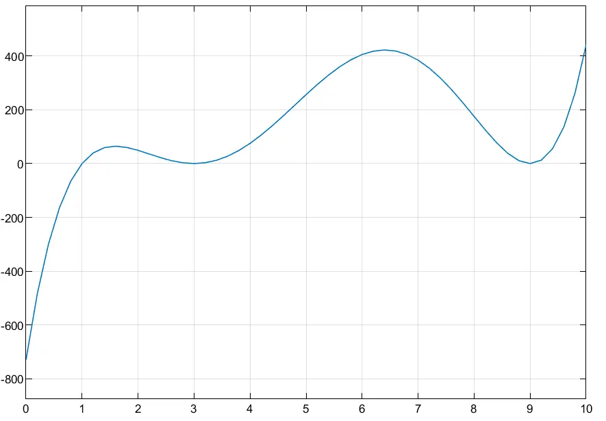
FIGURE.2

11. Thus from the above figure we can observe that how the value of function is changing w.r.t time.

EXAMPLE MODEL:

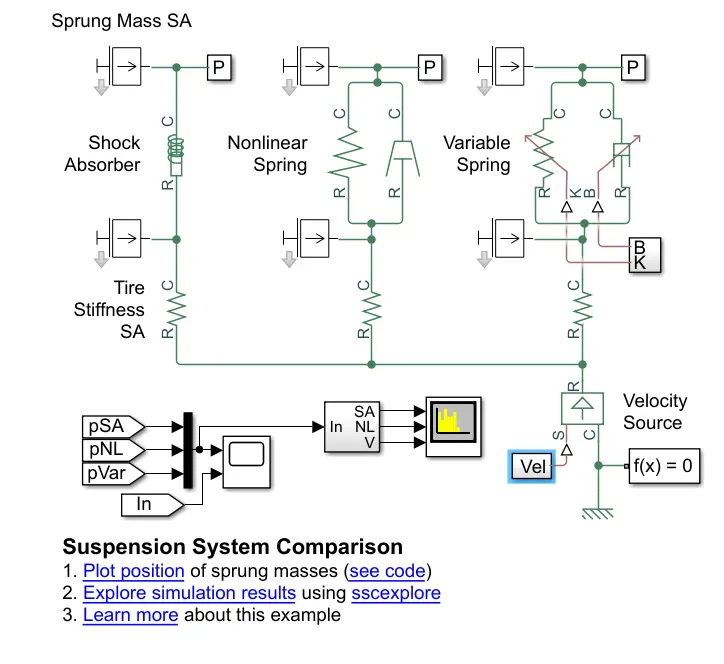
FIGURE.3

1. This example shows a testbed containing three sets of springs and dampers excited by the same oscillating velocity source.
2. The first uses the Shock Absorber block and includes linear stiffness and damping. Optional friction and hard stops are not used.
3. The second shock absorber uses a Nonlinear Translational Spring and a Nonlinear Translational Damper specified by symmetric polynomials.
4. The third uses a Variable Translational Spring and Variable Translational Damper. The spring constant is varied during the simulation using open loop control and the damping coefficient adjusts to ensure critical damping is achieved.
5. From the above example

i) The Objective the simulation is to observe how the three set of springs are excited by the same oscillating velocity source.

Here the velocity applied for all three is same .

Here the Tire Stiffness, Sprung mass and Unsprung mass are same for all three.

Here the Stiffness and Damping for each suspension system is different. For Shock absorber it changes linearly w.r.t displacement, for Non-Linear Spring it changes non-linearly w.r.t displacement and for variable spring it changes continuously.

ii) From the below results we can observe that, for low velocity the shock absorber and variable spring act similarly but the non-linear spring has slightly more negative sprung mass position. Now for medium velocity, the shock absorber and the non-linear show similar unequal positions of sprung mass i.e. the body is keeping on jumping up and down but in the case of variable spring there is a sudden jump and then the position of sprung mass constant i.e. it is keeping the body stable. Now at higher velocities there is small changes in shock absorbers and non-linear spring but the variable spring shows nearly constant values for the sprung mass position. So we can conclude at as the velocities increase the load is also increased so at higher loads variable spring is giving good output, at medium and small loads shock absorbers and non-linear spring are also giving good results but variable spring is giving better results at these velocities also. We can also see that when velocities are zero there are changes in the shock absorber and non-linear spring but the variable spring is constant for the sprung mass position.

So for smaller loads shock absorbers and non-linear spring can be used but for higher loads variable springs is better than other two.

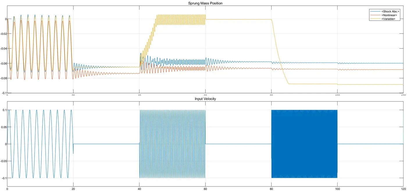
FIGURE.4

iii) Velocity source is created by multiplying sine wave and pulse generator. By observing the below diagram we can see three sets of sine wave block and pulse generator block are multiplies individually and then all there product outputs are added together and converted into physical quantity. Now here set of sine wave and pulse generator represents each type of velocity i.e. first set represents slow velocity, second set represents medium velocity and third set represents high velocity. These different types of velocities are achieved by changing the sine type parameter and frequency parameter in sine wave block and by changing phase delay parameter in the pulse generator block. By changing these parameters we can achieve different velocities and all these velocities together are given as input to all three suspension systems.

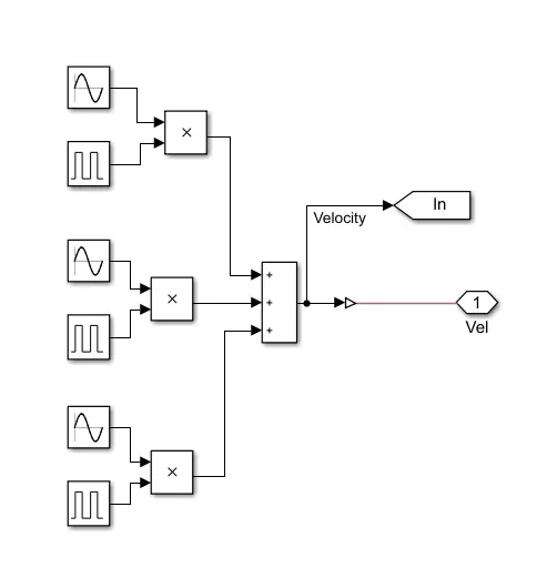
FIGURE.5

CONCLUSIONS:

1. Thus all the objectives are achieved successfully.
2. Similar kind of approach can be used to plot ant type of function using Simulink.
3. Various other examples can be studied and understood in the similar manner in Simulink.