Project

AIM:

To carry out a system level simulation of an All-Terrain Vehicle (ATV).

THEORY:

ALL-TERRAIN VEHICLE(ATV):

An all-terrain vehicle (ATV), also known as a quad, as defined by the American National Standards Institute (ANSI) is a vehicle that travels on low-pressure tires, with a seat that is straddled by the operator, along with handlebars for steering control. As the name implies, it is designed to handle a wider variety of terrain than most other vehicles. Although it is a street-legal vehicle in some countries, it is not street-legal within most states, territories, and provinces of Australia, the United States or Canada.

By the current ANSI definition, ATVs are intended for use by a single operator, although some companies have developed ATVs intended for use by the operator and one passenger. These ATVs are referred to as tandem ATVs.

The rider sits on and operates these vehicles like a motorcycle, but the extra wheels give more stability at slower speeds. Although most are equipped with three or four wheels, six-wheel models exist for specialized applications. Multiple-user analogues with side-by-side seating are called utility terrain vehicles (UTVs) or side-by-sides to distinguish the classes of vehicle. Both classes tend to have similar powertrain parts. Engine sizes of ATVs currently for sale in the United States (as of 2008 products) range from 49 to 1,000 cc (3.0 to 61 cu in).

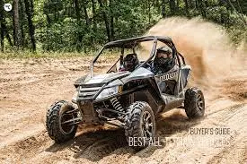
FIGURE.1

OBJECTIVE:

To prepare a technical report explaining the model properties & comments on the results.

SIMULINK MODEL:

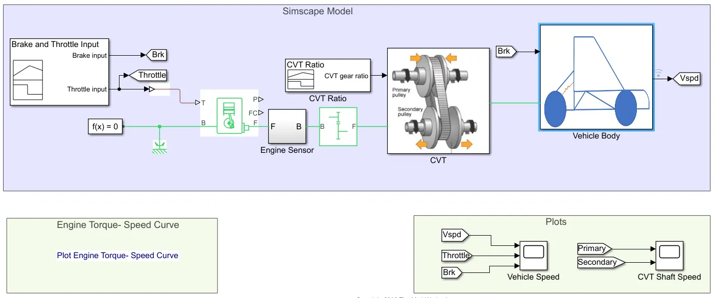
FIGURE.2

EXPLANATION:

1. The above model is a Baja ATV model with Continuously Variable Transmission (CVT).
2. Here first block connected is a ‘Signal Builder Block’ which is named as ‘Brake and Throttle Input’ where two input signals are generated, one for Brake and another for Throttle.

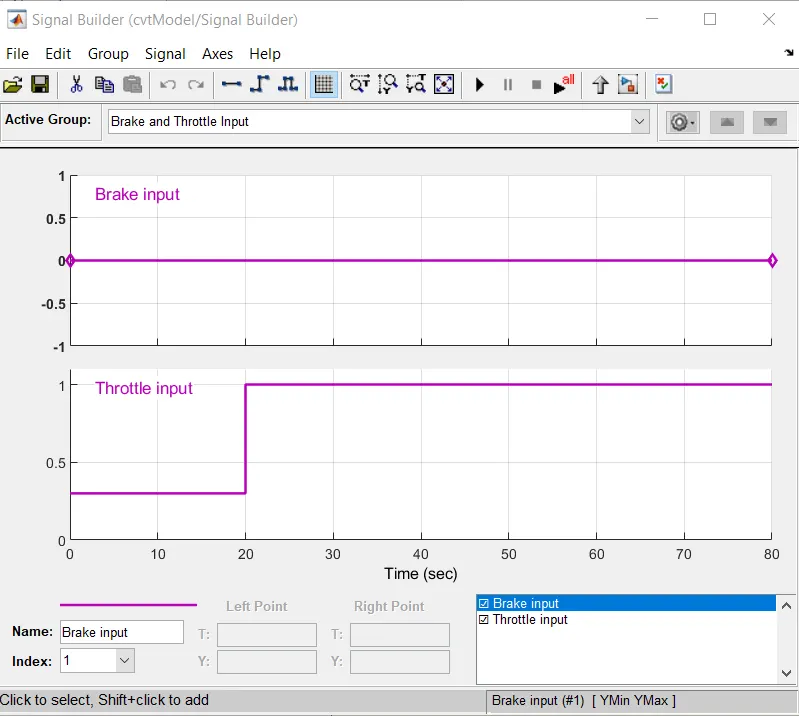
FIGURE.3

3. Now the throttle input signal from the ‘Brake and Throttle Input’ is connected to the ‘Generic Engine Block’, which represents a simple I.C. engine. This throttle input is connected to ‘T’ port of the engine block which is the throttle port for the engine.
4. Port ‘B’ is connected to a ‘Mechanical Rotational Reference’ which acts like a fixed point for a rotating part. Then this is connected to a ‘Solver Configuration Block’. Now port ‘F’ represents the crank shaft of the engine, which is the output of the engine block. Ports ‘P’ and ‘FC’ are physical signal output ports through which engine power and fuel consumption rate are reported.
5. Since we need only crank shaft to be connected with gear box, we have only connected port ‘F’ and left other ports unconnected.
6. Then port ‘F’ of engine block is connected to port ‘F’ of ‘Engine Sensor’. This ‘Engine Sensor’ is a sub system which consists of Simscape blocks to observe output angular velocity of the engine shaft.

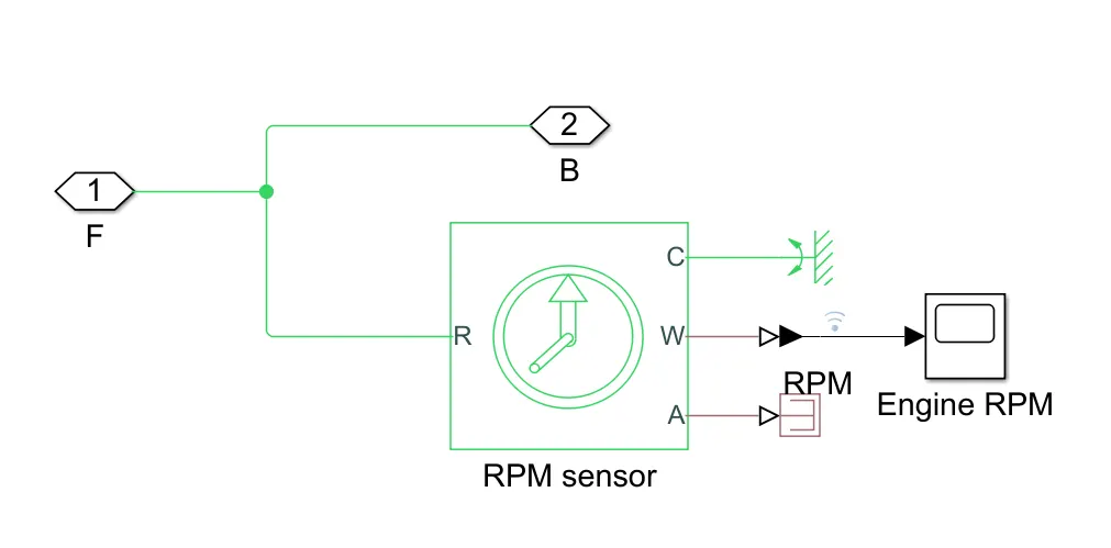
FIGURE.4

7. By double clicking the ‘Engine Sensor Block’ we can observe the above figure, in this sub system, a ‘Ideal Rotational Motion Sensor Block’ is used and it is connected to a ‘Scope Block’ to get the velocity readings. Ports R and C are mechanical rotational conserving ports, and ports W and A are physical signal output ports for velocity and angular displacement, respectively. Since we need only velocity, we have connected it to ‘Scope Block’ and angular displacement in connected to a terminator block which terminates the output.
8. Two Physical Modeling Connection Port are used to create output and input ports for this subsystem.
9. Now the output of this sub system is connected to a ‘Simple Gear Block’ which represents one gear system of a CVT gear, this block is connected to a ‘CVT Sub System’ which consists of a variable gear system.

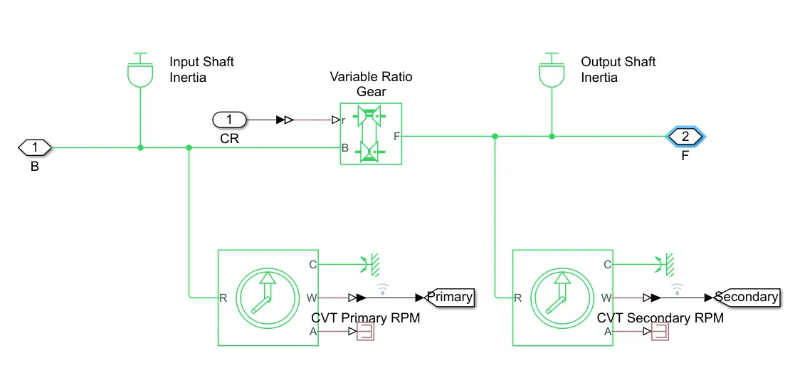
FIGURE.5

10. In this sub-system, first the simple gear block which is connected, is connected to a ‘Inertia Block’ where the block positive direction is from its port to the reference point. This means that the inertia torque is positive if the inertia is accelerated in the positive direction.
11. Then further this simple gear block is connected to one port of the ‘Variable Ratio Transmission Block’ which represents a variable ratio gearbox like CVTs, in this block the port ‘r’ defines the ratio of input to output angular shaft velocities.
12. To give values for this port, an ‘Signal Builder Block’ is used which is given as input to the sub system. The signal here gives the input to ‘r’ port thus defining the variable gear ratio.

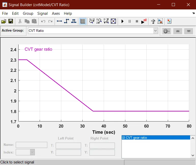
FIGURE.6

13. Now the output of this ‘Variable Ratio Transmission’ is connected to a physical modelling connection port which will act as output port of the Sub-System. The ‘Variable Ratio Transmission’ is also connected by a ‘Inertia Block’ and both the gears are also connected to ‘Ideal Rotational Motion Sensor Block’ to monitor the RPM at each gear systems.
14. Now the output of this CVT subsystem is connected to input of ‘Vehicle body’ subsystem, which represents whole vehicle.

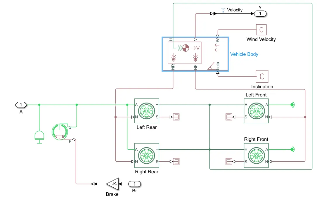
FIGURE.7

15. In this subsystem the input is connected to a ‘Tire Block’ where port ‘A’ is the mechanical rotational conserving port for the wheel axle. Connection H is the mechanical translational conserving port for the wheel hub through which the thrust developed by the tire is applied to the vehicle.
16. It is connected to two tire blocks which are considered as rear wheel which drive the vehicle. They are connected to ‘Inertia Block’ and ‘Double-Shoe Brake Block’ also. Input for the brake block is connected to the signal builder block which was created at starting as model and named as ‘Brake and Throttle Input’.
17. Now these two rear tyres are connected to two tire blocks with represent the two front wheels. All these four wheels are now connected to ‘Vehicle Body Block’ which represents a two-axle vehicle body in longitudinal motion. The block accounts for body mass, aerodynamic drag, road incline, and weight distribution between axles due to acceleration and road profile. The vehicle can have the same or a different number of wheels on each axle. Optionally include pitch and suspension dynamics or additional variable mass and inertia. The vehicle does not move vertically relative to the ground.
18. Ports ‘NR’ and ‘NF’ are normal forces acting on rear and front tires, port ‘beta’ represents the inclinations on the road which is connected to a ‘PS Constant Block’ which gives constant physical signal representing constant inclination. Port ‘H’ is a mechanical translation motion port which is connected to the tires for translation motion.
19. Port ‘W’ is physical signal for headwind speed which is also connected to ‘PS Constant Block’, now port ‘V’ is the velocity of the vehicle which is the output of the ‘Vehicle Body Block’ which is also output of the subsystem.
20. Now this output of the ‘Vehicle Body Block’ is connected to a ‘Goto Block’
21. Now ‘From Block’ of the whole model are now connected to ‘Scope Blocks’ to observe the results of the system. Velocity from the Vehicle Body subsystem, brake and throttle signals from the signal builder block are connected to one Scope Block and Output of two gears in the CVT subsystem are connected to another Scope Block representing their RPM.

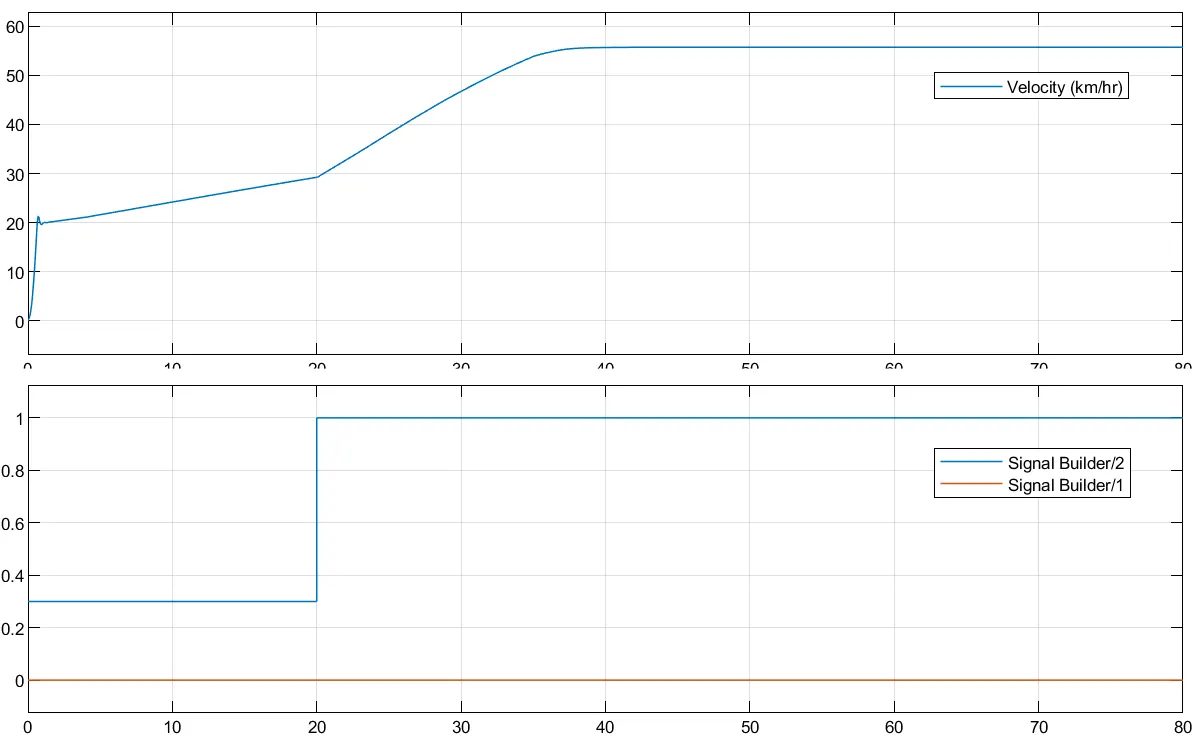
FIGURE.8

22. From the above result we can observe that as the throttle of the vehicle is increasing the speed of the vehicle is also increasing. Initially as the throttle is constant the speed is rising slowly, once the throttle is increased to maximum the speed also increased and continued at constant speed.

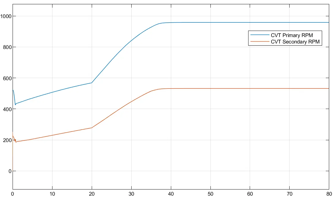
FIGURE.9

23. The above figure are the results of the RPM from the gear system in the CVT subsystem. If we observe the graph the rpm of the primary gear system that is output of ‘Simple Gear Block’ is the blue curve which has higher rpm, but the secondary gear system that is the output of ‘Variable Transmission Block’ is has less rpm and this is due to loss of power. Always the output power is less than the input power due losses. This graph represents the same, how the power is transmitted in the CVT system.

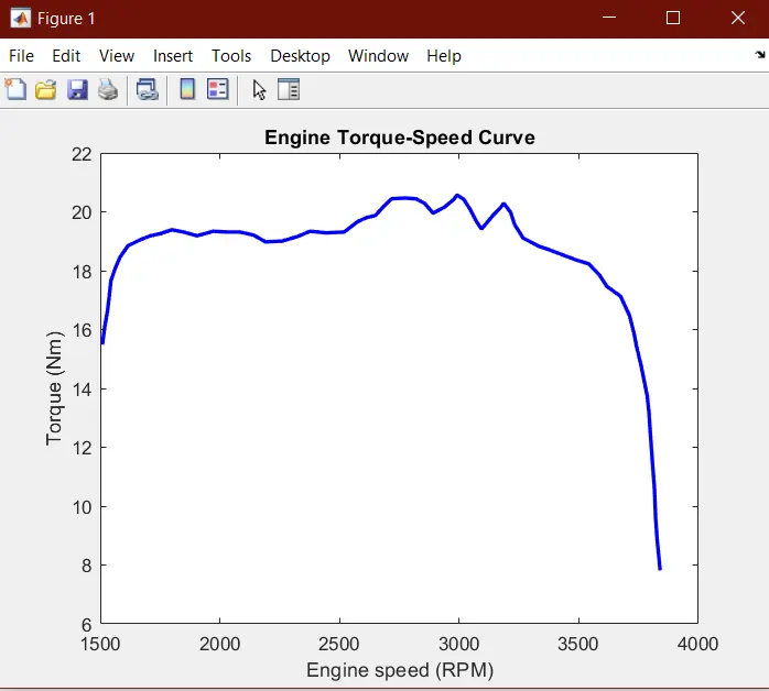
FIGURE.10

24. Now when we click on the plot link in the model, we get the above graph. We can observe in the above graph that at initial speeds the torque is more and as the speed is increasing the torque is also increasing upto certain speed and at high speeds the torque is vey less. This is because torque is inversely proportional to speed at high speeds. At high speeds there is no need of torque to move the vehicle so it is less.

MODEL WITH DASHBOARD:

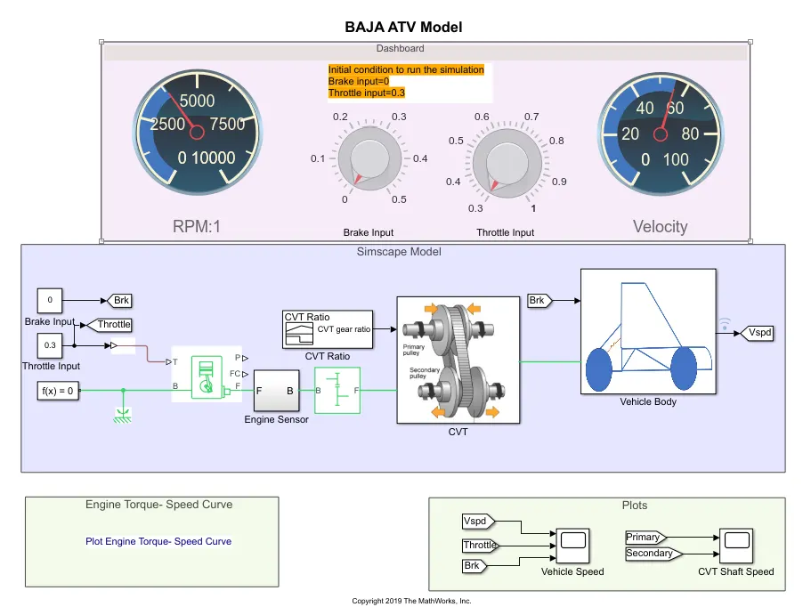
Figure.11

1. The above model is same that of previous model but with some differences in inputs and has better representation than the previous one.
2. Once we run the program, we can see the different RPMs and speed in a speedometer like blocks known as ‘Custom Gauge Block’ which displays the values. We can also change the inputs like throttle and braking values while the model is running using a ‘Knob Block’ manually.
3. To assign these types of inputs first a ‘Constant Block’ is used to give input as Throttle and Brake, then these blocks are linked with the ‘Knob Block’ separately and the minimum and maximum values are set in this block.
4. Similarly, the RPM from the ‘Scope Block’ named as ‘CVT Shaft Speed’ is linked with the first ‘Custom Gauge Block’ named as ‘RPM:1’ which displays RPM values and the speed from the ‘Scope Block’ named as ‘Vehicle Speed’ is linked with the second ‘Custom Gauge Block’ named as ‘Velocity’ which displays vehicle speed values.
5. Thus, we can monitor the results by changing the input values manually according to our need.

CONCLUSION:

1. Thus, system level simulation is successfully done for a All-Terrain Vehicle(ATV).
2. Similar approach can be used to understand other vehicle models and systems.