Final Project: Electric Rickshaw modelling

AIM:

To create a detailed MATLAB model of an electric Rickshaw.

THOERY:

Electric rickshaws (also known as electric tuk-tuks or e-rickshaws or toto or e-tricycles) have been becoming more popular in some cities since 2008 as an alternative to auto rickshaws and pulled rickshaws because of their low fuel cost, and less human effort compared to pulled rickshaws. They are being widely accepted as an alternative to petrol/diesel/CNG auto rickshaws. They are three-wheelers powered by an electric motor ranging from 650 to 1400 Watts. They are mostly manufactured in India and China, only a few other countries manufacture these vehicles. Battery-run rickshaws could be a low-emitter complementary transport for the low-income people, who suffer most from a lack of transport facility, if introduced in a systematic manner according to experts.

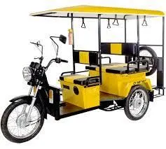
FIGURE.1

OBJECTIVE:

For any three cycles, to show energy consumption, temperature rise and of motor and controller for 100 km constant speed driving at 45 kmph.

SOLUTION:

MAKING OF MATLAB-SIMULINK MODEL:

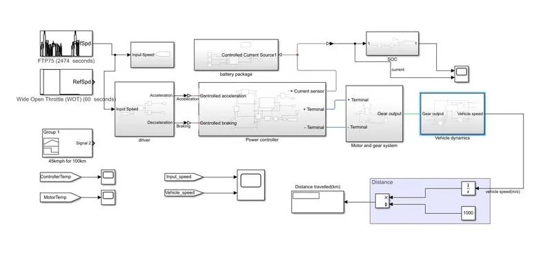
FIGURE.2

To make the Matlab model we need the following system blocks:

1. Driver Subsystem:

This is the system where the inputs from driver are given the system in terms of speed. To represent the driver input speed, we have used three different blocks i.e. ‘DRIVE CYCLE BLOCK’, ‘WIDE OPEN THROTTLE BLOCK’ and ‘SIGNAL BUILDER BLOCK’.

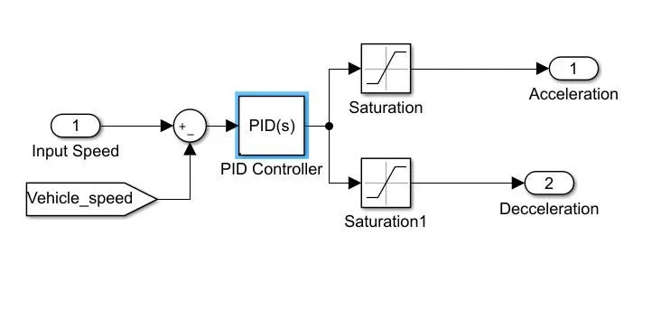
FIGURE.3

Here we can see that the input speed is fed with feedback of the final vehicle speed and this sum is sent to the ‘PID Controller Block’ so that PID controller will decided whether it has to accelerate or decelerate the vehicle.

2. Power Controller:

This is the system where, according to the PID controller’s output, the power controller i.e. the set of IGBTs work. Here using “PWM SIGNAL BLOCK’ we are sending at what signal and rate the IGBTs have to work to match the input speed. Here these IGBTs are represented using a ‘H-BRIDGE BLOCK’ where the output is calculated as current required to match the input speed.

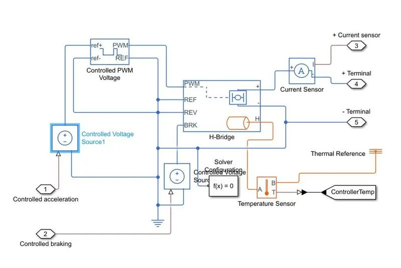
FIGURE.4

Here we can see that first the output from PID controller is connected to a ‘CONSTANT VOLTAGE SOURCE BLOCK’ where it will provide constant voltage regardless the value of current. For both acceleration and deceleration, a separate ‘CONSTANT VOLTAGE BLOCK’ is provided so even though there are fluctuations in the current due to change in acceleration and decelerations the voltage will be constant. Then this change in acceleration is send to the ‘PWM BLOCK’ so that it can send the appropriate frequency for the ‘H-BRIDGE BLOCK’. Now from ‘H_BRIDGE BLOCK’ the current is given as output of this system. Before this, the h-bridge is connected to ammeter so that we can measure the current. Similarly this H-Bridge is also connected to the ‘TEMPERATURE SENSOR’ so that we can measure the temperature of H-Bridge while it is working.

3. Battery Package:

This sub-system represents the battery of the vehicle. This system will help to monitor the condition of the battery in terms of voltage and current.

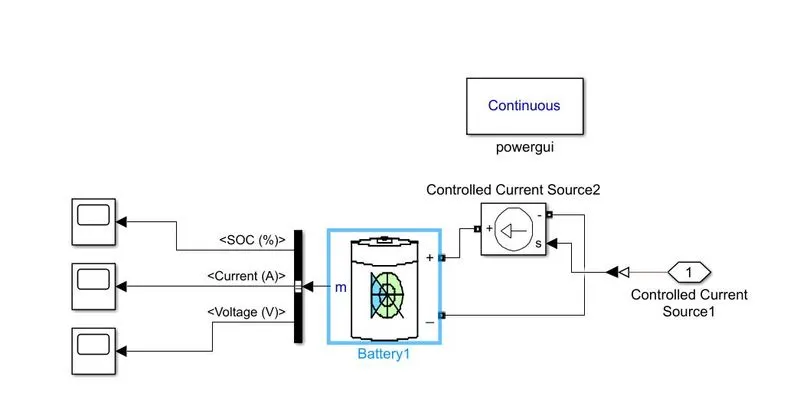
FIGURE.5

Here we can see that the current signals from ‘H_BRIDGE’ is connected to this system where first this current signals are converted into physical currents. Using this signals we then have connected it to the ‘BATTERY BLOCK’ where according to these current signal the battery block shows us how much current is used from the battery pack to the match the input current signals, along with this will also show the SOC and voltage change of the battery.

4. Motor and Gear:

This sus-system represents the working of motor of the electric rickshaw. This is the transmission part of the vehicle.

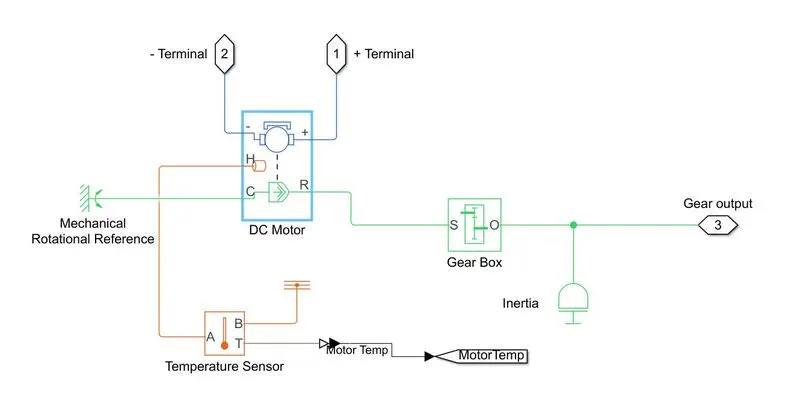
FIGURE.6

Here we can see that the output from the H-Bridge i.e. positive and negative points are now connected to ‘DC MOTOR BLOCK’ in this system. This block represents the working of DC Motor. Then this DC Motor block is connected to the ‘GEAR BOX BLOCK’ where the motor will transmit the power to vehicle through this gear box block. Here certain gear ratio is applied. This DC Motor block is also connected to a ‘TEMPERATURE SENSOR BLOCK’ where the motor temperature is measured.

5. SOC:

Here system shows how the energy from battery is used and how the current is drawn.

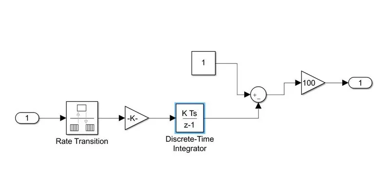
FIGURE.7

Here we can see that using the ‘RATE TRANSITION BLOCK’ we have used the current signals from H-Bridge to read values at higher rate and then by using the ‘DISCRETE-TIME INTEGRATOR BLOCK’ we have calculated the soc of battery at each input speed.

6. Vehicle Dynamics:

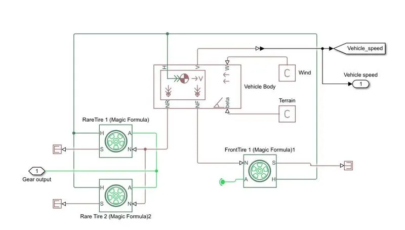
This sub-system shows the all the force calculations that act on the vehicle.

FIGUER.8

Here we can observe that first there is an arrangement of the wheels of the vehicle for which we have used ‘TIRE BLOCK’. Then these tire blocks are connected with each other and then these are connected to the ‘VEHICLE DYNAMIC BLOCK’ where all the forces acting on the vehicle are calculated. Thus, the output of this is the final speed of the vehicle. Then this vehicle speed is connected to the integration block where speed is integrated and the respective distance is calculated.

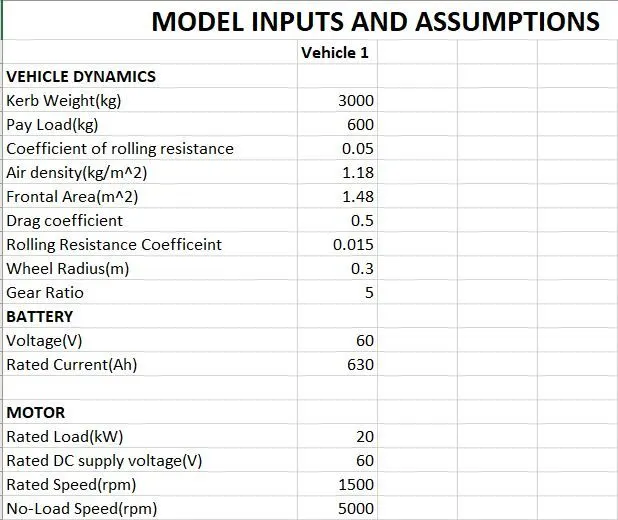
ASSUMED INPUT VALUES:

RESULTS:

I) USING FTP75 DRIVE CYCLE AS INPUT:

First, we have run the model using FTP75 drive cycle and we got the following results:

Vehicle Speed Graph:

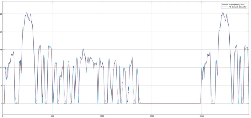
FIGURE.9

In the above results we can see that the vehicle speed is almost same as the input reference speed graph. That means that the system is correctly trying to match the input speed, thus providing required speed as output.

SOC Graph:

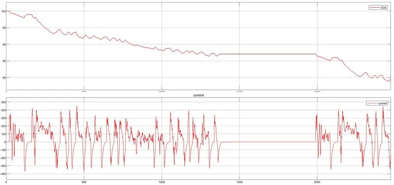
FIGURE.10

Here we can observe how battery is discharging at each instant of speed when the model simulation is running. We can observe how the current is drawn at each instant to match the input speed.

II) USING WIDE OPEN THROTTLE AS INPUT:

Second, we have run the model using WOT drive cycle and we got the following results:

Vehicle Speed Graph:

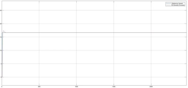
FIGURE.11

In the above graph we can see that vehicle speed has reached the speed that was given in the wide-open throttle inputs. First the speed raised from 0 to the speed that was set as input. Once it reached the top speed there is a small jump and then the speed is maintained constant then afterwards thus following the input speed.

SOC Graph:

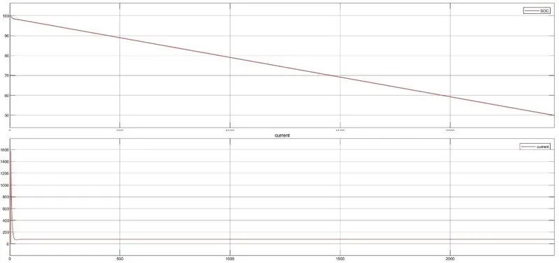
FIGURE.12

Here we can see the battery charge has come from 100% to 50% at the end of the simulation. In the current graph also since initially vehicle needed more current to reach the top speed so the current consumed also is high in the initial and then its constant since the speed is constant once the top is reached and is constant.

III) USING SIGNAL BUILDER AS INPUT:

Third, we have run the model using Signal Builder drive cycle and we got the following results:

Vehicle Speed Graph:

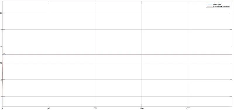
FIGURE.13

Here we can see similar kind of results that of what we have seen in WOT graphs. Here we have just changed the top speed and it has been achieved successfully.

SOC Graph:

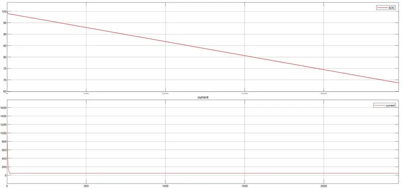
FIGURE.14

Here the change in SOC and Current in the battery is similar to that of WOT graphs. The current initially drawn is high as the vehicle has to achieve the top speed.

THERMAL RESULT:

1. I) For FTP75 Drive Cycle:

Controller Temperature Graph:

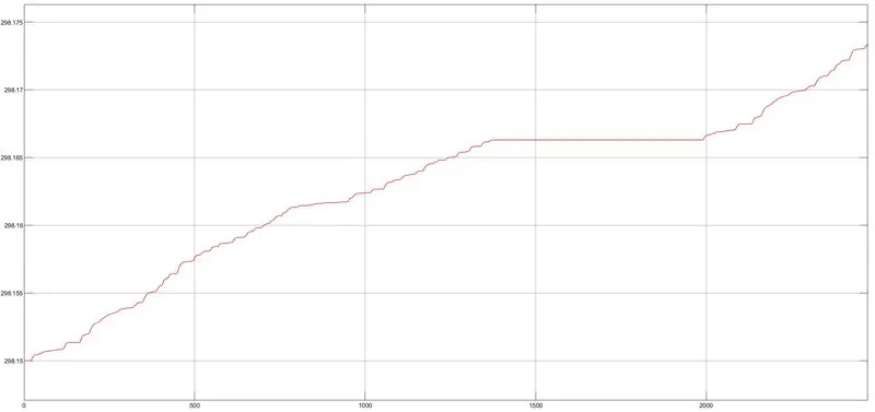
FIGURE.15

Here we can as the vehicle is running according to the input speed the temperature of the Controller is also increasing according since it is being working all the time through out the symbol.

Motor Temperature Graph:

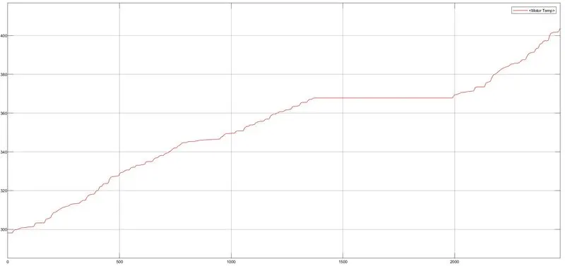
FIGURE.16

Here we can see that the graph is similar to that of controller’s temperature graph. Here also since the motor is running continuously the temperature is also rising accordingly. Only difference is the values in the temperatures in the graphs.

1. II) For WOT Drive Cycle:

Controller Temperature Graph:

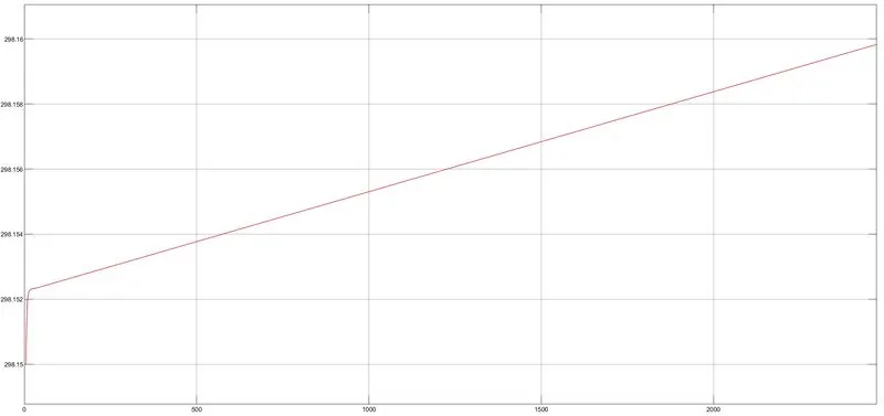
FIGURE.17

Here we can see the temperature initial has increased rapidly since the vehicle was reaching top speed. and then it constantly increased after it has reached constant speed.

Motor Temperature Graph:

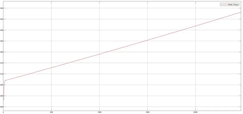
FIGURE.18

Here we can see that the graph is similar to that of controller’s temperature graph. Here the graphs trend is similar to that of the Controller’s temperature. Only difference is the values in the temperatures in the graphs.

III) For Signal Builder Drive Cycle:

Controller Temperature Graph:

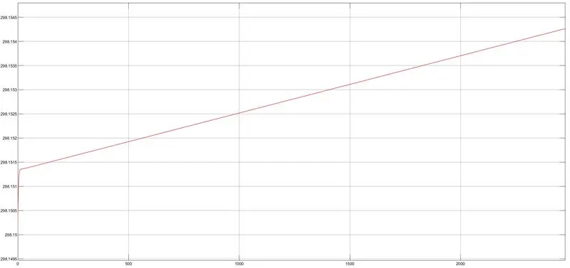
FIGURE.19

Here we can observe similar graph to that of WOT thermal graph. But her the temperature values are different since the top speed id different in both the cases. Here also initial temperature rise is high since the vehicle has to achieve the top speed and then once the speed is constant the temperature rise also constant.

Motor Temperature Graph:

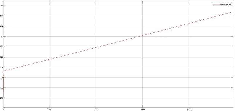
FIGURE.20

Here we can see that the graph is similar to that of controller’s temperature graph. Here the graphs trend is similar to that of the Controller’s temperature. Only difference is the values in the temperatures in the graphs.

CONCLUSIONS:

1. Thus, the Matlab model of Electric Rikshaw was created and simulated successfully.
2. Similar kind of approach can be followed to create similar Matlab models.

Link Of Model File:- https://drive.google.com/drive/folders/1NdyKCmYGlQbZQE8FU-Gft1FL1a5E8PUd?usp=sharing