Curve Fitting using MATLAB

Q: Write code to fit a linear and cubic polynomial for the Cp data.

Plot the linear and cubic fit curves along with the raw data points. Title and axes labels are a must, legends could be shown if necessary.

Write a code to show splitwise method.

Explain the parameters used to measure the fitness characteristics for both the curves.

A: Curve Fitting is a process of constructing a curve or mathematical functions, that has the best fit to a series of data points, possibly subjected to constraints. Curve Fitting includes interpolation and smoothing techniques.

It is highly effective in the mathematical modelling of some natural processes.

The Curve Fit is used for various applications. For example, finding the population in future by keeping the future time and inserting previous data in a country.

• Linear polynomial means the highest degree in the polynomial equation is 1. The fit made using this equation is known as a linear fit.

Example of a linear polynomial is y = mx + c

Where, 'm' is the slope and 'c' is the intercept. 'y' and 'x' are the dependent or independent variables respectively.

• Cubical polynomial means the highest degree in the polynomial equation is 3. The fit made using this equation is known as cubical fit.

Example of a cubical polynomial is y = ax^3 + bx^2 + cx + d

a, b, c, d are coefficients. 'y' and 'x' are the dependent or independent variables respectively.

Definitions and their syntaxes:

• polyfit: p = polyfit(x, y, n) returns the coefficients for a polynomial p(x) of degree n that is the best fit (in a least-squares sense) for the data in y. The coefficients in p are in descending powers, and the length of p is n+1.
  
  p(x)=p1*(x^n)+p2(x^(n−1))+...+pn*x+pn+1.
  
  
• polyval: p = polyfit(p, x) evaluates polynomial p at each point. The argument p is a vector of length n + 1, whose elements are the coefficients (in descending powers) of an nth-degree polynomial
  
  p(x)=p1*(x^n)+p2(x^(n−1))+...+pn*x+pn+1.
  
  
• Centering and Scaling: This centering and scaling transformation improves the numerical properties of both the polynomial and the fitting algorithm.
  
  Syntax: [p, S, mu] = polyfit(x, y, n) also returns 'mu', which is a two-element vector with centering and scaling values. mu(1) is mean(x), and mu(2) is std(x). Using these values, polyfit centres x at zero and scales it to have a unit standard deviation.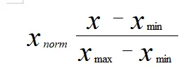
  
  
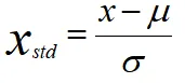
  Where σ = standard deviation and μ = mean.
  
  
• Sum of Squared Errors(SSE): ∑(i = 1 to n) = Error(i)^2
  
  
• R-square explains how successful the fit is explaining the data.
  
  R-square = SSR/SST where, SSR = ∑(i = 1 to n) (f(x(i)) - mean)^2
  
  SST = SSR + SSE , where SSR = sum of squares of regression.
  
  
• Adjusted R-square is a normalising variation of R-square which neglects the variation of R-square due to insignificant independent variables.
  
  
  
• Root Mean Square Error (RMSE) = sqrt(SSE/n)
  
  

Note: Goodness of fit can be calculated in both ways. First one is by writing the above formulas in code and the second one is calculating directly using curve fitting toolbox. Here, we use curve fitting toolbox to find the goodness of fit by calculating all terms.

Curve fitting toolbox:

In this toolbox, we won't use any 'polyfit' or 'polyval' options for curve fitting. This toolbox is not only used for 2D-plots, it is also used for 3D- plots. When we include values of Z-axis with both X and Y-axis values, it gives 3D-plots.

In this toolbox, we also get values directly. values like coefficients, SSE, R-square, Adjusted R-square, RMSE. These values are shown automatically when we insert values.

There are multiple options in this toolbox. We can also generate code from this toolbox, results can be displayed in workspace etc.

Code procedure:

1. In this code, we are creating three curves. One is for original data, second is a linear curve fitting and third is cubic fit.
   
   
2. Add statements as shown below.
   
   clear all
   
   close all
   
   clc
   
   
3. Now we need to load the file from the file manager of PC. Make sure that data file should be in the same directory of the code file. Assign file data to a variable, 'cp_data'.
   
   cp_data = load('data');
   
   
4. Data contains two columns of values. The first column represents temperature and the next column represents specific heat. Assign the column values as 'temperature' and 'cp'.
   
   temperature = cp_data(:, 1) ;
   
   cp = cp_data(:, 2) ;
   
   
5. Till now we got the values of original data for plotting the curve. We need to find the curve fitting for the linear and cubic equation.
   
   
6. A linear polynomial equation is y = ax + b. 'y' and 'x' are dependent and independent variables. It represents the function of y = f(x). 'a' and 'b' are the coefficients of the equation. For curve fitting of a polynomial equation, we use 'polyfit' and 'polyval' commands which are in-built tools in MATLAB.
   
   Add 'polyfit' command with values of 'temperature' and 'cp' with a degree of polynomial 1. Since we are finding for linear equation, we use 1. This gives values of coefficients and assigned to a variable 'co_eff1'.
   
   co_eff1 = polyfit(temperature, cp, 1) ;
   
   Use 'polyval' command for finding the new cp values for prediction. Add new co-efficient and temperature values. These values are assigned to a variable 'predicted_cp1'.
   
   predicted_cp1 = polyval(co_eff1, temperature) ;
   
   
7. Now we should find the values for cubic polynomial equation. A cubic polynomial equation is y = ax^3 + bx^2 + cx + d. 'y' and 'x' are dependent and independent variables. It represents the function of y = f(x). 'a', 'b', 'c' and 'd' are the coefficients of the equation.
   
   Add 'polyfit' command with values of 'temperature' and 'cp' with a degree of polynomial 3. Since we are finding for cubic equation, we use 3. This gives values of coefficients and assigned to a variable 'co_eff3'.
   
   co_eff3 = polyfit(temperature, cp, 3) ;
   
   Use 'polyval' command for finding the new cp values for prediction. Add new co-efficient and temperature values. These values are assigned to a variable 'predicted_cp3'.
   
   predicted_cp3 = polyval(co_eff3, temperature) ;
   
   
8. Here, we plot curves for three values with temperature i.e., cp, predicted_cp1, predicted_cp3. Plotting original curve with linewidth 3 and red colour. Add statements for predicted values also using blue and green colour. Use hold on command for plotting 3 curves in one figure.
   
   plot(temperature, cp, 'linewidth', 3, 'color', 'r')
   
   hold on
   
   plot(temperature, predicted_cp1, 'linewidth', 3, 'color', 'b')
   
   hold on
   
   plot(temperature, predicted_cp3, 'linewidth', 3, 'color', 'g')
   
   
9. Add hold off statements for terminating intermixing of plots for next. Adding these commands helps us to get a good figure and also avoids intermixing.
   
   hold off
   
   
10. Add labels for X and Y-axis as 'Temperature [K]' and 'Specific Heat [kJ/kmol-K]' respectively. Adding a title for the plot.
    
    xlabel('Temperature [K]')
    
    ylabel('Specific Heat [kJ/kmol-K]')
    
    title('Plot of curve fitting original vs linear vs cubic')
    
    
11. To avoid confusion in the output figure among the three curves, we should represent each of it with names.
    
    legend('original data', 'linear fit', 'cubic fit')
    
    'legend' is a command which is used to represent curves.
    
    
12. Run the program.
    
    

Code:

clear all
close all
clc

% Loading data from the file manager
cp_data = load('data');
temperature = cp_data(:,1);
cp = cp_data(:,2);

% Finding values for linear equation
% linear equation equation y = ax + b

co_eff1 = polyfit(temperature, cp, 1);
predicted_cp1 = polyval(co_eff1, temperature);

% Finding values for cubic equation
% cubic equation y = ax^3 + bx^2 + cx + d

co_eff3 = polyfit(temperature, cp, 3);
predicted_cp3 = polyval(co_eff3, temperature);

% Plotting linear and cubic fit with original fit

plot(temperature, cp, 'linewidth', 3, 'color', 'r')
hold on
plot(temperature, predicted_cp1, 'linewidth', 3, 'color', 'b')
hold on
plot(temperature, predicted_cp3, 'linewidth', 3, 'color', 'g')
hold off

% Adding labels for both axes

xlabel('temperature [K]')
ylabel('specific heat [kJ/kmol-K]')
title('Plot of curve fitting original vs linear vs cubic')

% Representation of curves

legend('original curve', 'linear fit', 'cubic fit')

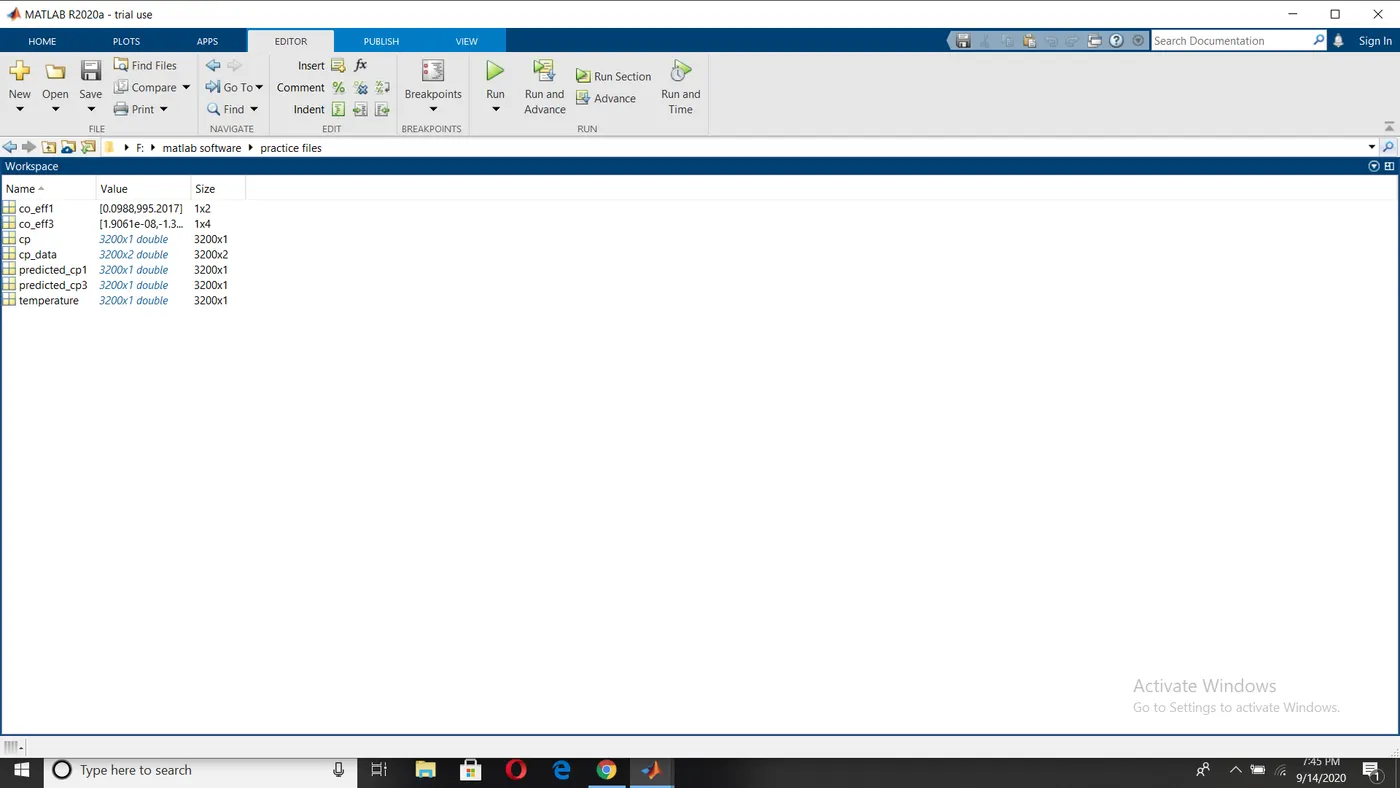
Workspace:

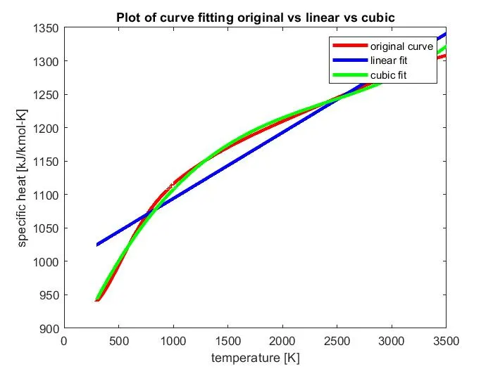
Output figure: We get three curves in a single figure.

Splitwise method: In this method, we split the values of temperatures and specific heats into 4 equal parts.

1. Open MATLAB and click new script.
   
   
2. Add statements as shown below.
   
   clear all
   
   close all
   
   clc
   
   
3. Now we need to load the file from the file manager of PC. Make sure that data file should be in the same directory of the code file. Assign file data to a variable, 'cp_data'.
   
   cp_data = load('data');
   
   
4. Data contains two columns of values. The first column represents temperature and the next column represents specific heat. Assign the column values as 'temperature' and 'cp'.
   
   temperature = cp_data(:, 1) ;
   
   cp = cp_data(:, 2) ;
   
   
5. Add 'polyfit' command with values of 'temperature' and 'cp' with a degree of a polynomial 2. This gives values of coefficients and assigned to a variable 'co_eff'.
   
   co_eff = polyfit(temperature, cp, 2) ;
   
   Use 'polyval' command for finding the new cp values for prediction. Add new co-efficient and temperature values. These values are assigned to a variable 'predicted_cp'.
   
   predicted_cp = polyval(co_eff, temperature) ;
   
   
6. For curve fitting, we need to divide temperature and specific heat values. Here, we divide into four equal parts. Add statements for dividing temperature.
   
   temp11 = cp_data(1 : 800, 1);
   
   temp12 = cp_data(801 : 1600, 1);
   
   temp13 = cp_data(1601 : 2400, 1);
   
   temp14 = cp_data(2401 : 3200, 1);
   
   
7. Now, we divide specific heat values.
   
   cp11 = cp_data(1 : 800, 2);
   
   cp12 = cp_data(801 : 1600, 2);
   
   cp13 = cp_data(1601 : 2400, 2);
   
   cp14 = cp_data(2401 : 3200, 2);
   
   
8. Using 'polyfit' for finding the coefficient of each curve.
   
   coeff11 = polyfit(temp11, cp11, 1);
   
   coeff12 = polyfit(temp12, cp12, 1);
   
   coeff13 = polyfit(temp13, cp13, 1);
   
   coeff14 = polyfit(temp14, cp14, 1);
   
   
9. Use 'polyval' command.
   
   predict_cp11 = polyval(coeff11, temp11);
   
   predict_cp12 = polyval(coeff12, temp12);
   
   predict_cp13 = polyval(coeff13, temp13);
   
   predict_cp14 = polyval(coeff14, temp14);
   
   
10. For curve fitting, we need to divide temperature and specific heat values. Here, we divide into four equal parts. Add statements for dividing temperature.
    
    temp21 = cp_data(1 : 800, 1);
    
    temp22 = cp_data(801 : 1600, 1);
    
    temp23 = cp_data(1601 : 2400, 1);
    
    temp24 = cp_data(2401 : 3200, 1);
    
    
11. Now, we divide specific heat values.
    
    cp21 = cp_data(1 : 800, 2);
    
    cp22 = cp_data(801 : 1600, 2);
    
    cp23 = cp_data(1601 : 2400, 2);
    
    cp24 = cp_data(2401 : 3200, 2);
    
    
12. Using 'polyfit' for finding the coefficient of each curve.
    
    coeff21 = polyfit(temp21, cp21, 3);
    
    coeff22 = polyfit(temp22, cp22, 3);
    
    coeff23 = polyfit(temp23, cp23, 3);
    
    coeff24 = polyfit(temp24, cp24, 3);
    
    
13. Use 'polyval' command.
    
    predict_cp21 = polyval(coeff21, temp21);
    
    predict_cp22 = polyval(coeff22, temp22);
    
    predict_cp23 = polyval(coeff23, temp23);
    
    predict_cp24 = polyval(coeff24, temp24);
    
    
14. Plot curves of original vs linear in figure 1. For good notation, give linewidth 2 for original and for linear give 3.
    
    figure(1)
    
    plot(temp, cp, 'r', 'linewidth', 3)
    
    hold on
    
    plot(temp11, predict_cp11, 'b', temp12, predict_cp12, 'b', 'linewidth', 2)
    
    hold on
    
    plot(temp13, predict_cp13, 'b', temp14, predict_cp14, 'b', 'linewidth', 2)
    
    hold off
    
    To get plots in a single figure, we use 'hold on' and 'hold off' commands.
    
    
15. Add labels for X and Y-axis as temperature [K] and 'specific heat [kJ/kmol-K]'
    
    xlabel('temperature [K]')
    
    ylabel('specific heat [kJ/kmol-K]')
    
    title('Plot of curve fitting original vs linear-split')
    
    
16. Use legend command for representing curves in the figure.
    
    legend('original', 'linear-split')
    
    
17. Plot curves of original vs cubic in figure 1. For good notation, give linewidth 2, for original and for cubic, give 3.
    
    figure(1)
    
    plot(temp, cp, 'r', 'linewidth', 3)
    
    hold on
    
    plot(temp21, predict_cp21, 'b', temp22, predict_cp22, 'b', 'linewidth', 2)
    
    hold on
    
    plot(temp23, predict_cp23, 'b', temp24, predict_cp24, 'b', 'linewidth', 2)
    
    hold off
    
    To get plots in a single figure, we use 'hold on' and 'hold off' commands.
    
    
18. Add labels for X and Y-axis as temperature [K] and 'specific heat [kJ/kmol-K]'
    
    xlabel('temperature [K]')
    
    ylabel('specific heat [kJ/kmol-K]')
    
    title('Plot of curve fitting original vs cubic-split')
    
    
19. Use legend command for representing curves in the figure.
    
    legend('original', 'cubic-split')
    
    
    
20. Run the program.
    
    
21. Since we used the degree of the polynomial is 3, we get warnings in the command window. The warning shows that degree is given more and reduce it or try centering and scaling. Even warnings have appeared, plots are executed.
    
    

Code:

close all
clear all
clc

% Loading data
cp_data = load('data');
temp = cp_data(:,1);
cp = cp_data(:,2);

% Splitting values from the data into 4 equal parts for linear fit
% Obtaining temperatures

temp11 = cp_data(1:800,1);
temp12 = cp_data(801:1600,1);
temp13 = cp_data(1601:2400,1);
temp14 = cp_data(2401:3200,1);

% Obtaining specific heat values

cp11 = cp_data(1:800,2);
cp12 = cp_data(801:1600,2);
cp13 = cp_data(1601:2400,2);
cp14 = cp_data(2401:3200,2);

% Finding values for linear expressions

coeff11 = polyfit(temp11,cp11,1);
coeff12 = polyfit(temp12,cp12,1);
coeff13 = polyfit(temp13,cp13,1);
coeff14 = polyfit(temp14,cp14,1);

% Finding predicted cp values

predict_cp11 = polyval(coeff11,temp11);
predict_cp12 = polyval(coeff12,temp12);
predict_cp13 = polyval(coeff13,temp13);
predict_cp14 = polyval(coeff14,temp14);

% Splitting values from the data into 4 equal parts for cubic fit
% Obtaining temperatures

temp21 = cp_data(1:800,1);
temp22 = cp_data(801:1600,1);
temp23 = cp_data(1601:2400,1);
temp24 = cp_data(2401:3200,1);

% Obtaining specific heat values

cp21 = cp_data(1:800,2);
cp22 = cp_data(801:1600,2);
cp23 = cp_data(1601:2400,2);
cp24 = cp_data(2401:3200,2);

% Finding values for linear expressions

coeff21 = polyfit(temp21,cp21,3);
coeff22 = polyfit(temp22,cp22,3);
coeff23 = polyfit(temp23,cp23,3);
coeff24 = polyfit(temp24,cp24,3);

% Finding predicted cp values for cubic fit

predict_cp21 = polyval(coeff21,temp21);
predict_cp22 = polyval(coeff22,temp22);
predict_cp23 = polyval(coeff23,temp23);
predict_cp24 = polyval(coeff24,temp24);

% Plotting for original and linear fit with separate linewidths
figure(1)
plot(temp,cp,'r', 'linewidth',3)
hold on
plot(temp11,predict_cp11,'b',temp12, predict_cp12,'b','linewidth',2)
hold on
plot(temp13,predict_cp13,'b',temp14, predict_cp14,'b','linewidth',2)
hold off

% Adding labels

xlabel('temperature [K]')
ylabel('specific heat [kJ/kmol-K]')
title('Plot of curve fitting original vs linear-split')

% Adding names for curves

legend('original', 'linear-split')

% Plotting for original and linear fit with separate linewidths

figure(2)
plot(temp,cp,'r', 'linewidth',3)
hold on
plot(temp21,predict_cp21,'b',temp22, predict_cp22,'b','linewidth',2)
hold on
plot(temp23,predict_cp23,'b',temp24, predict_cp24,'b','linewidth',2)
hold off

% Adding labels

xlabel('temperature [K]')
ylabel('specific heat [kJ/kmol-K]')
title('Plot of curve fitting original vs cubic-split')

% Adding names for curves

legend('original', 'cubic-split')

Workspace:

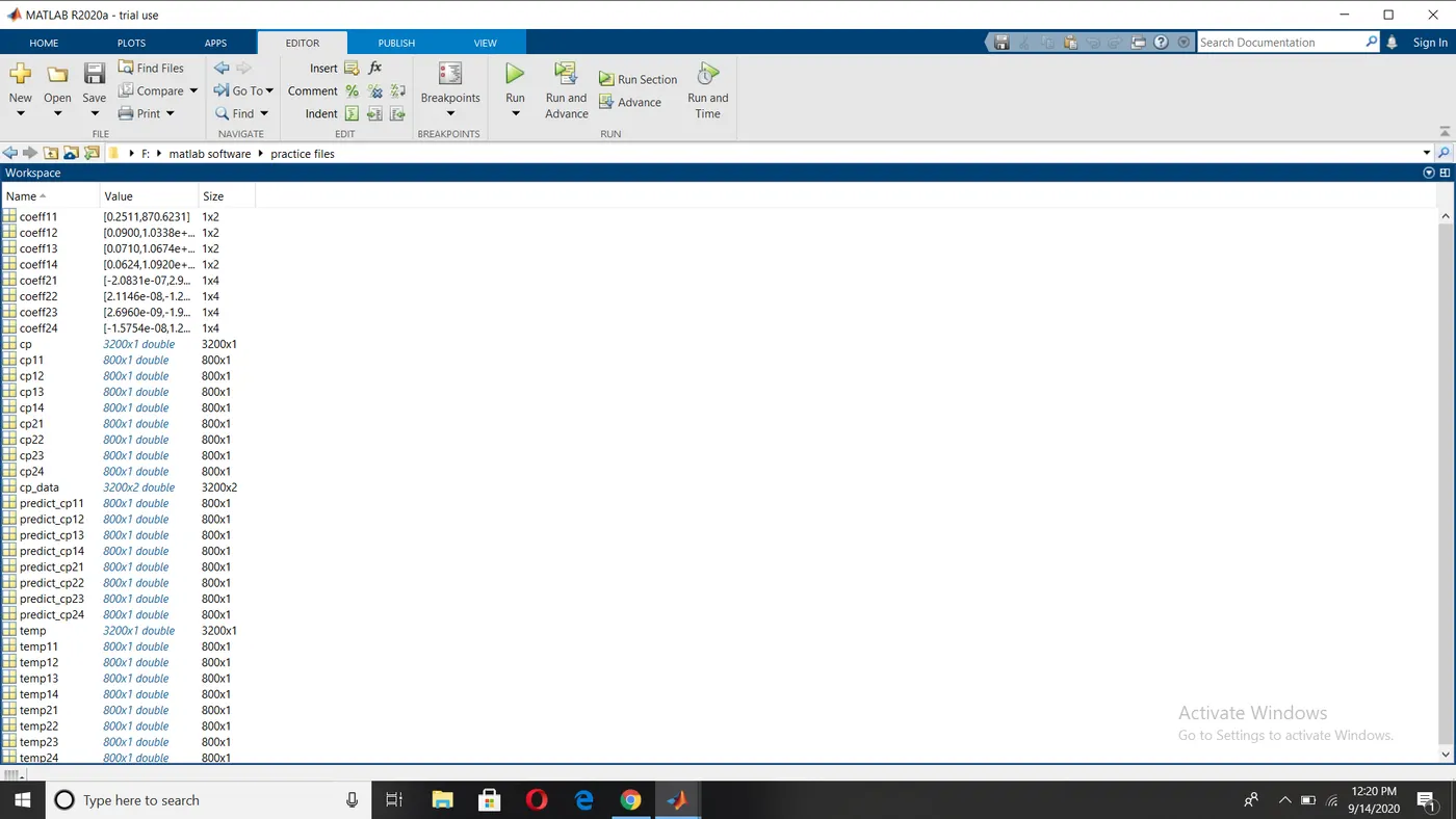
Output in the command window:

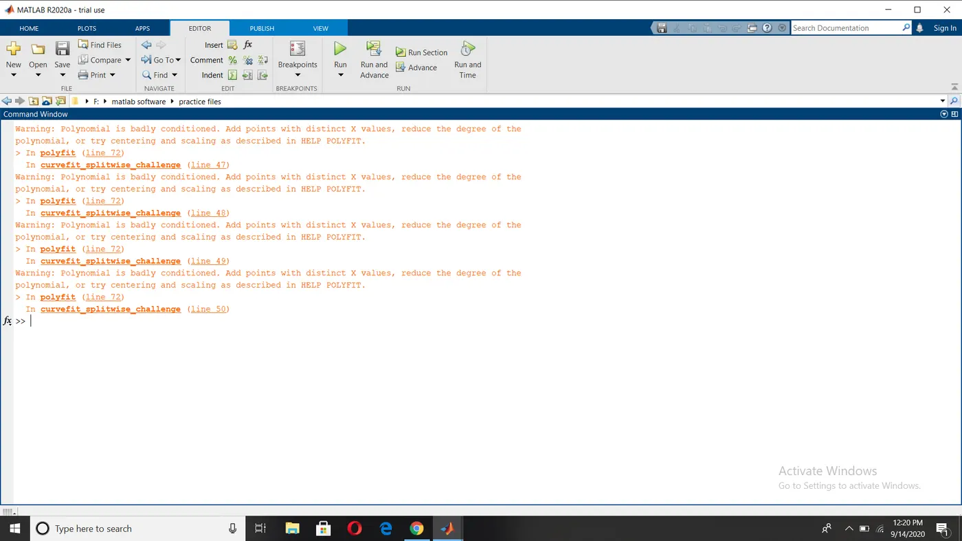
Figure 1: Plot of original vs linear fit by using splitwise method.

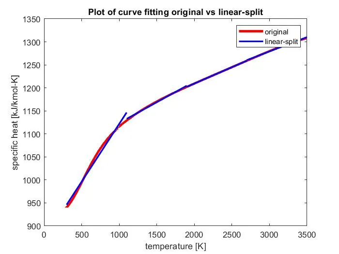
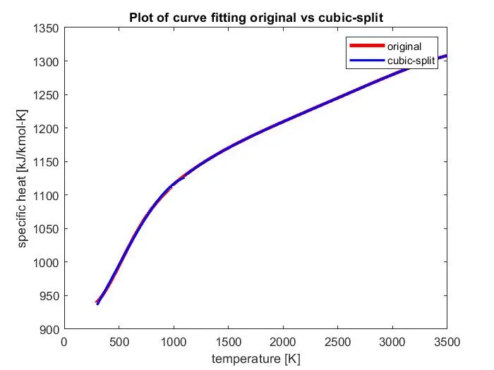
Figure 2: Plot of original vs cubic fit by using splitwise method.

To avoid warnings, we use centering and scaling option which can be done in two ways. The first method is manually writing formulas(which are given in the description) in the code and the second method is selecting the option in curve fit toolbox.

Finding the best fit using command fit toolbox.

Using Curve fit toolbox:

To find, the goodness of fit we use curve fit toolbox. We load the data in the main window of MATLAB.

1. Open curve fit toolbox either by typing 'cftool' in the command window or selecting 'curve fitting toolbox' option from Apps for checking whether it is present in your software while installing.
   
   
2. Open the new script in MATLAB. Add statements as follows.
   
   clear all
   
   close all
   
   clc
   
   
3. Type 'cftool' to open curve fit toolbox.
   
   cftool
   
   
4. Load data from the file manager. assign data values to a variable 'cptdata'
   
   cptdata = load('data')
   
   
5. Since the cptdata contains two values i.e., temperature and specific heat, we divide them and assign to new variables.
   
   temp = cptdata(:, 1)
   
   cp = cptdata(:, 2)
   
   
6. Run the code for opening and toolbox. Save the file.
   
   
7. A new window opens which is curve fit toolbox. At the top left corner, give a name for the type of fit. Here we do 2 types of fits i.e., linear and cubic compared with the original. Add the fit name as 'linear fit'. Select the X data as temp and Y data as cp.
   
   
8. Select polynomial option and under it give degree as 1. Tick auto fit option. We get a curve below in the window. Results in the left side of the window.
   
   
9. Coefficients and goodness of fit values are shown.
   
   
   

Code in MATLAB editor:

clear all
close all
clc

cftool

cptdata = load('data')
temp = cptdata(:, 1)
cp = cptdata(:, 2)

Curve fitting toolbox: The below figure contains inputs and outputs. Results for the goodness of fit are displayed at the left and curves are displayed at the right bottom.

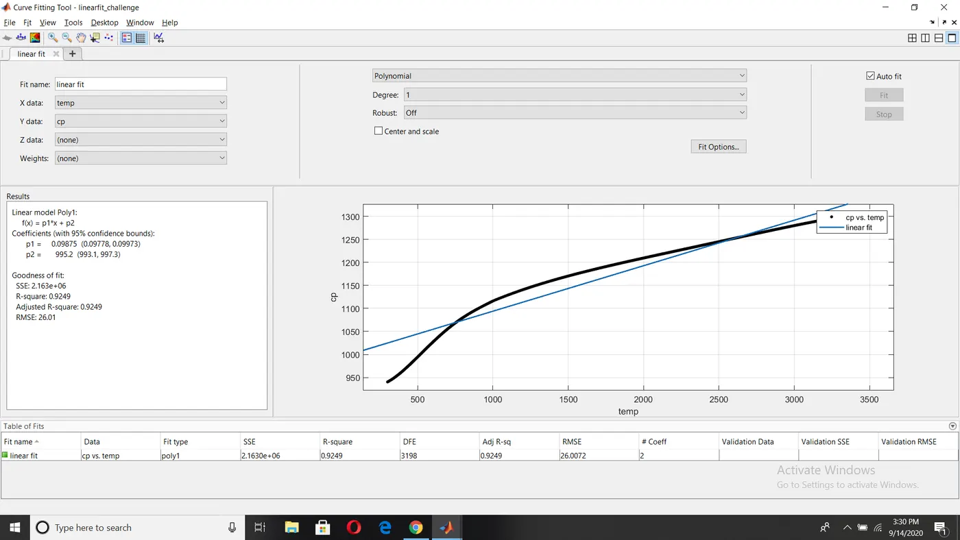
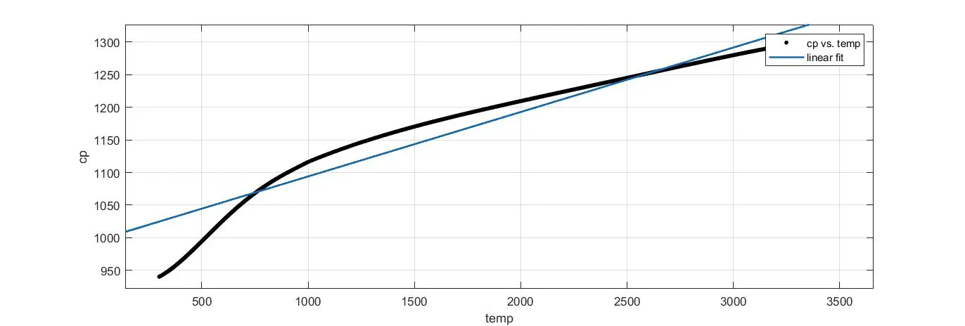
A plot of original vs linear fit: We can observe that linear fit vs original curve.

Cubic fit vs original fit:

1. Open new session(click new tab) in curve fitting toolbox.
   
   
2. At the top left corner, give a name for the type of fit. Add the fit name as 'cubic fit'. Select the X data as temp and Y data as cp.
   
   
3. Select polynomial option and under it give degree as 3. Tick auto fit option. We get a curve below in the window. Results in the left side of the window.
   
   
4. Coefficients and goodness of fit values are shown.
   
   
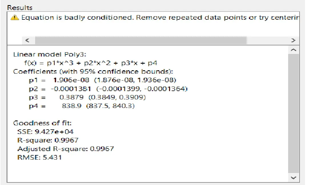
5. If it shows warning in the results tab, select centering and scaling option. This option improves the numerical properties of both polynomial and the fitting algorithm.
   
   

Cubic fit in the toolbox: The below figure contains inputs and outputs. Results for the goodness of fit are displayed at the left and curves are displayed at the right bottom.

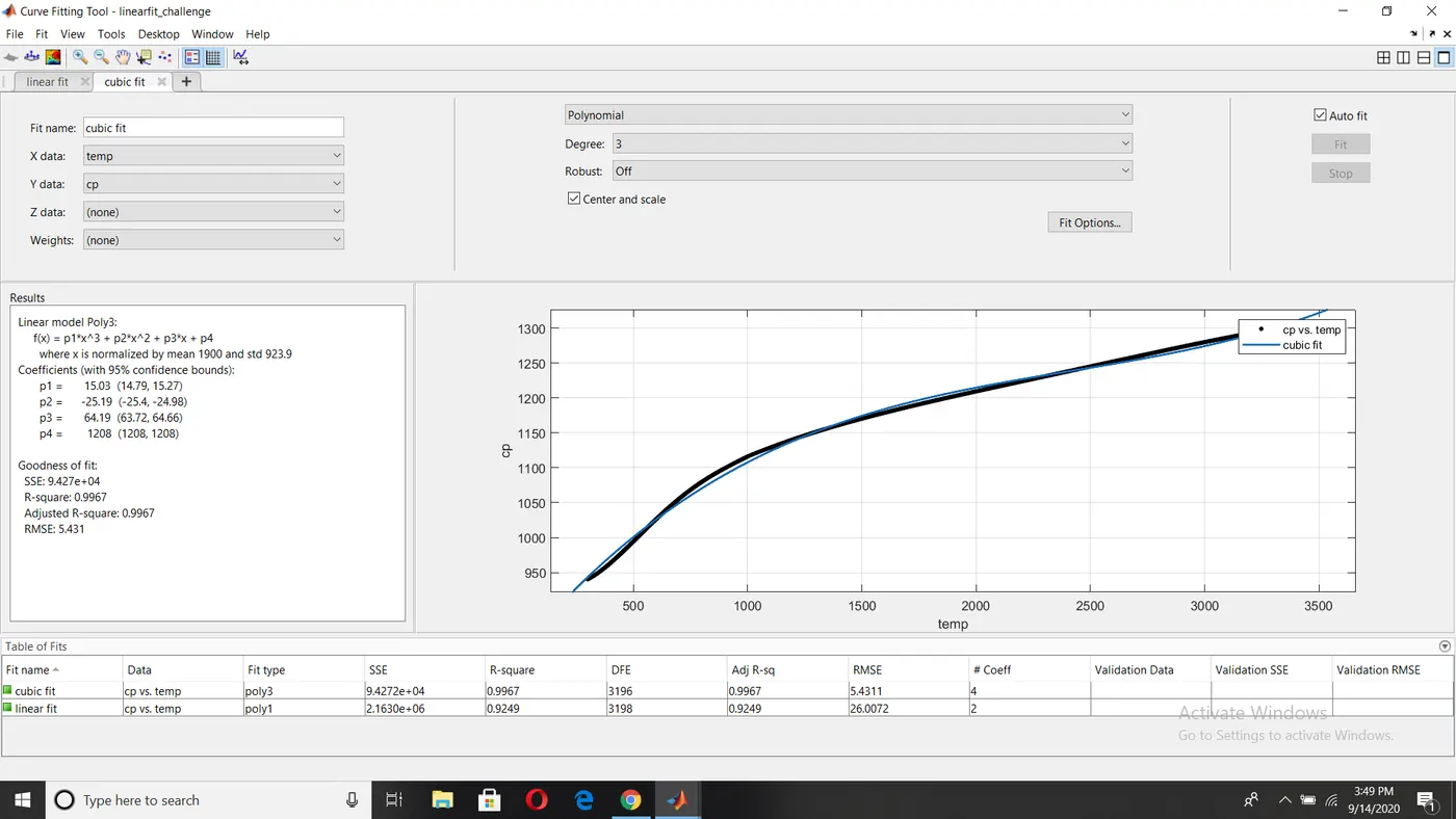
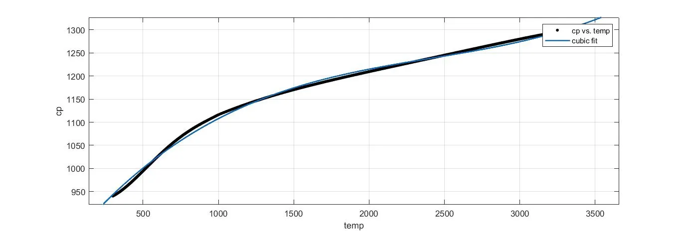
Plot for original vs cubic fit: We can observe that cubic fit almost equal to the original curve.

Note:

We know R-square value ranges from 0 to 1. R-square value for the first fit is 0.9249 and for the second is 0.9967. By this, we can ay that cubic fit is good for the above data. In the parameters of the above solution like SSE, R-square, Adjusted R-square, RMSE are calculated for finding the best fit. These parameters help find the best and also errors in the curves.

References: I referred mathsworks site for detail syntaxes and explanation.

https://skill-lync.com/projects/Curve-Fitting-and-criterion-to-choose-best-fit-41860

https://skill-lync.freshdesk.com/support/solutions/articles/43000584172

https://en.wikipedia.org/wiki/Curve_fitting

https://en.wikipedia.org/wiki/Linear_regression

Data file: Link for cp and temperature data

Q1: How to make fit perfectly?

A1: To make a fit perfectly, we should use a higher degree polynomial equation. The fit becomes perfect where it is almost equal to the original curve.

Q2: How to get the best fit?

A2: Use centering and scaling to make the best fit. By using values like SSE, R-square, Adjusted R-square, RMSE we can find the best fit. By reducing errors we can find best. We can also use splitwise method. Minimising distance between two curves also can be done to make the fit better.

Q3: What could be done to improve cubic fit?

A3: Using centering and scaling option we improve cubic fit. This can be done by using the formula in code or using an option in the toolbox.

Points to remember:

• Use polyfit and polyval commands according to their syntaxes and insert
• The data file should from the same directory. While loading data, the file name must be given correctly.
  
  
• The legend names sequence should match with plot curves sequence.
  
  
• Give necessary expression in the toolbox. The degree should be given correctly to avoid warnings.
  
  
• Try the same colours for all divided plots in splitwise function.

Errors and rectification:

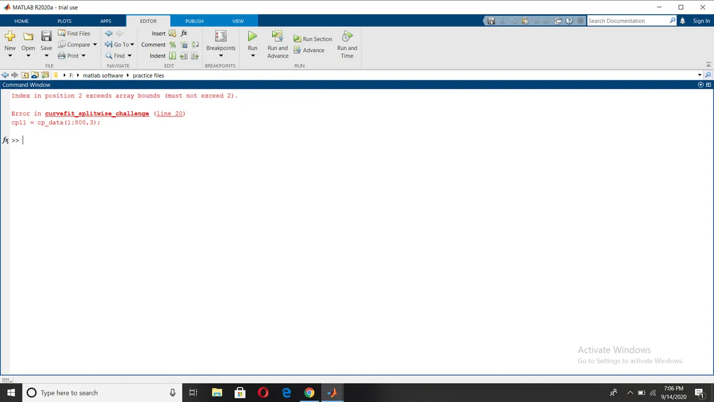
1. An error occurred when we give the wrong index(i.e., more than the matrix). We know the column matrix for the above example does not exceed 2. If we give 3, below error is an error. Write carefully while giving matrix index values.
   
   
   
   
2. Warning displayed when the polynomial equation is given as 3 in curve fitting toolbox. It shows as below.
   
   
   

Conclusion: Therefore, the best fit is calculated and represented by using various commands. If we increase the degree of polynomial the more perfect fit for the data we get.