Curve fitting and checking the goodness of fit using MATLAB
Objective:
To write a code to perform curve fitting for the given Temperature vs Cp data and to check the goodness of the obtained curve.
Description:
Curve fitting is one of the most powerful and most widely used analysis tool. Curve fitting examines the relationship between one or more predictors (independent variables) and a response variable (dependent variable), with the goal of defining a "best fit" model of the relationship. Here, the function of Curve fitting method sounds similar to that of interpolation methods but both are apparently different.
Interpolation:
In Interpolation method we find a function satisfying `P(x_i) = f (x_i); i = 1, . . . , n` that allows us to approximate `f (x)` such that the function values between the data sets may be estimated or in a simple way Interpolation is a method of constructing new data points within the range of a discrete set of known data points.
Curve fitting
Curve fitting is the process of constructing a curve, or mathematical function, that has the best fit to a series of original data points possibly subject to constraints. The function does not have to pass through the original data points.
Interpolation vs curve fitting
Curve-fitting is when we have a dataset of scattered points and find a line (or curve) that best fits the general shape of the data.
Interpolation is when we have two points of data and want to know what a value between the two would be. Half way between would be their average, but if we want to know only a quarter of the way between the two, we'd have to interpolate.
Note: Curve fitting can involve either interpolation, where an exact fit to the data is required, or smoothing, in which a smooth function or a trend line is constructed that approximately fits the data
Here, the curve can be
1 Polynomials of degree n
2 Trigonometric
3 Exponential
In MATLAB, the function polyfit performs polynomial regression
Polyfit and Polyval
Matlab has two functions, polyfit and Polyval, which can quickly and easily fit a set of data points with a polynomial.
Polyfit is a Matlab function that computes a least squares polynomial for a given set of data. Polyfit generates the coefficients of the polynomial, which can be used to model a curve to fit the data.
Polyval evaluates a polynomial for a given set of x values. So, Polyval generates a curve to fit the data based on the coefficients found using polyfit.
How to Evaluate Goodness of Fit
After fitting data with one or more models, you should evaluate the goodness of fit. A visual examination of the fitted curve displayed in Curve Fitting app should be your first step. Beyond that there are 4 quantities which help us measure the goodness of fit criteria or how well the equation is representing the datapoints. They are:
1. The sum of squares due to error
2. R-square
3. Adjusted R-square
4. Root mean squared error (RMSE)
In this project I’m going to use R-square method to evaluate the goodness of the fit.
R-Square method:
This quantity that measures how successful the fit is in explaining the variation of the data. Put another way, R-square is the square of the correlation between the response values and the predicted response values. It is also called the square of the multiple correlation coefficient and the coefficient of multiple determination.
What that means in layman's terms is that the higher the value of R-square the better the fit, the lower it is the lousier the fit, R-square ranges from a value of 0 to 1
The value of R-square ranges from 0 (worst possible fit) – 1(best possible fit).
Formulae to calculate R-square
`SSR = sum(Predicted .C_p - Mean(C_p))^2`
`SSE = sum(Cp - Predicted.C_p)^2`
`SST = SSR + SSE`
`R^2 = (SSR)/(SST)`
where, SSR – Sum of Squares of Regression
SSE - Sum of Squares of Error
SST - Sum of Squares of Total
The ‘best’ fit has minimum error between Predicted curve and the given data points. Mostly, the acceptable range is between 0.95 – 1.
It is said to be a 'Perfect' fit if the value of R-square is equal to 1.
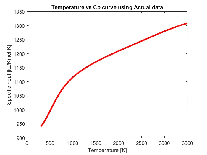
Let us look at the code to plot the curve between given Temperature and Cp values:
%------------------------------------------------------------------
clear all
close all
clc

data = load('data');                %Loading the data from the file

temp = data(:,1);                   %Retriving Temperature data
Cp = data(:,2);                     %Retriving Cp data

figure(1)
plot(temp,Cp,'r','linewidth',3)
xlabel('Temperature [K]')
ylabel('Specific heat [kJ/Kmol-K]')
title('Temperature vs Cp curve using Actual data')
%------------------------------------------------------------------
Output:
Matlab code to linear fit for the Cp data:
%--------------------------------------------------------------------------------
clear all
close all
clc

data = load('data');                %Loading the data from the file

temp = data(:,1);                   %Retriving Temperature data
Cp = data(:,2);                     %Retriving Cp data

%Curve fitting is done by using Split-wise method
start = 0;                          %Assigining dummy value for starting step
stop = 0;                           %Assigining dummy value for ending step
predicted_Cp=zeros(length(Cp),1);   %Assigining dummy values for Cp to be predicted
frequency = 3200;                   %Frequency of steps
n = 1;                              %Order of polynomial

for i = 1:length(Cp)/frequency

start = stop+1;                     %Assigining the value for starting step
stop = stop + frequency;            %Assigining the value for ending step

temp_step = temp(start:stop);       %Loading the values of temperature in between the range
cp_step = Cp(start:stop);           %Loading the values of Cp in between the range

[coeff] = polyfit(temp_step,cp_step,n); %To find the coeeficients
new_cp = polyval(coeff,temp_step);    %To find the value of Predicted Cp

%To merge all the values of predicted Cp in one matrix
predicted_Cp(start:stop) = predicted_Cp(start:stop)+ new_cp;

end

%To check the goodness of fit
SSR = sum(predicted_Cp - mean(Cp))^2;
SSE = sum(Cp - predicted_Cp)^2;
SST = SSR + SSE;
R2 = SSR/SST

figure(1)
plot(temp,Cp,'r','linewidth',1.5)
hold on
plot(temp,predicted_Cp,'b','linewidth',1.5)
xlabel('Temperature [K]')
ylabel('Specific heat [kJ/Kmol-K]')
legend('Actual Cp','Predicted Cp','location','northwest')
title(sprintf('Linear Curve Fit (1st Order) with R-Square value %f',R2))
%--------------------------------------------------------------------------------
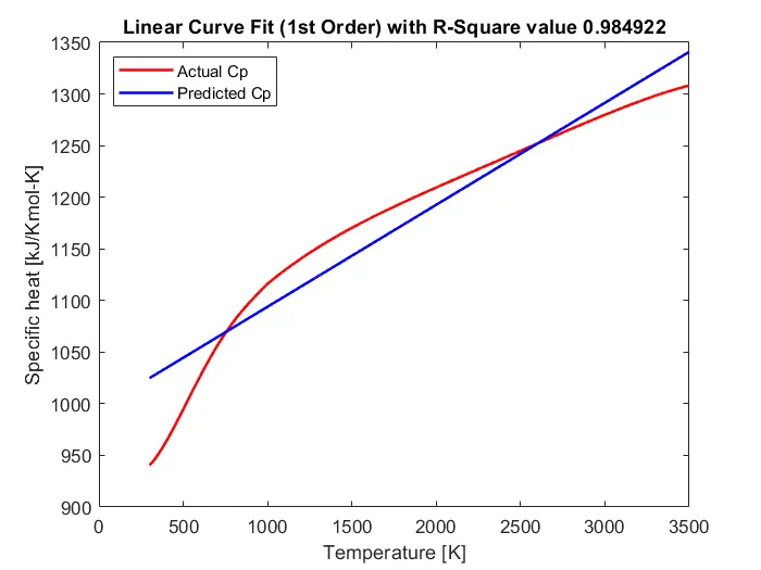
Output:
Matlab code to fit a cubic polynomial for the Cp data:
%--------------------------------------------------------------------------------
clear all
close all
clc

data = load('data');                %Loading the data from the file

temp = data(:,1);                   %Retriving Temperature data
Cp = data(:,2);                     %Retriving Cp data

%Curve fitting is done by using Split-wise method
start = 0;                          %Assigining dummy value for starting step
stop = 0;                           %Assigining dummy value for ending step
predicted_Cp=zeros(length(Cp),1);   %Assigining dummy values for Cp to be predicted
frequency = 3200;                   %Frequency of steps
n = 3;                              %Order of polynomial

for i = 1:length(Cp)/frequency

start = stop+1;                     %Assigining the value for starting step
stop = stop + frequency;            %Assigining the value for ending step

temp_step = temp(start:stop);       %Loading the values of temperature in between the range
cp_step = Cp(start:stop);           %Loading the values of Cp in between the range

[coeff] = polyfit(temp_step,cp_step,n); %To find the coeeficients
new_cp = polyval(coeff,temp_step);    %To find the value of Predicted Cp

%To merge all the values of predicted Cp in one matrix
predicted_Cp(start:stop) = predicted_Cp(start:stop)+ new_cp;

end

%To check the goodness of fit
SSR = sum(predicted_Cp - mean(Cp))^2;
SSE = sum(Cp - predicted_Cp)^2;
SST = SSR + SSE;
R2 = SSR/SST

figure(1)
plot(temp,Cp,'r','linewidth',1.5)
hold on
plot(temp,predicted_Cp,'b','linewidth',1.5)
xlabel('Temperature [K]')
ylabel('Specific heat [kJ/Kmol-K]')
legend('Actual Cp','Predicted Cp','location','northwest')
title(sprintf('Cubic Polynomial Curve Fit (3rd Order) with R-Square value %f',R2))
%--------------------------------------------------------------------------------
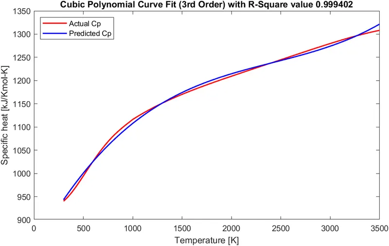
Output:
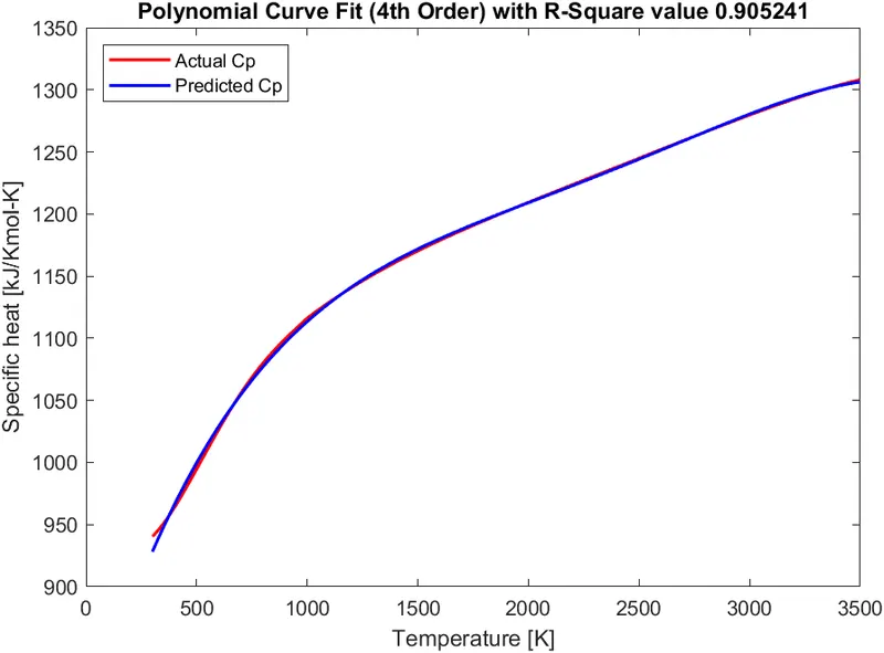
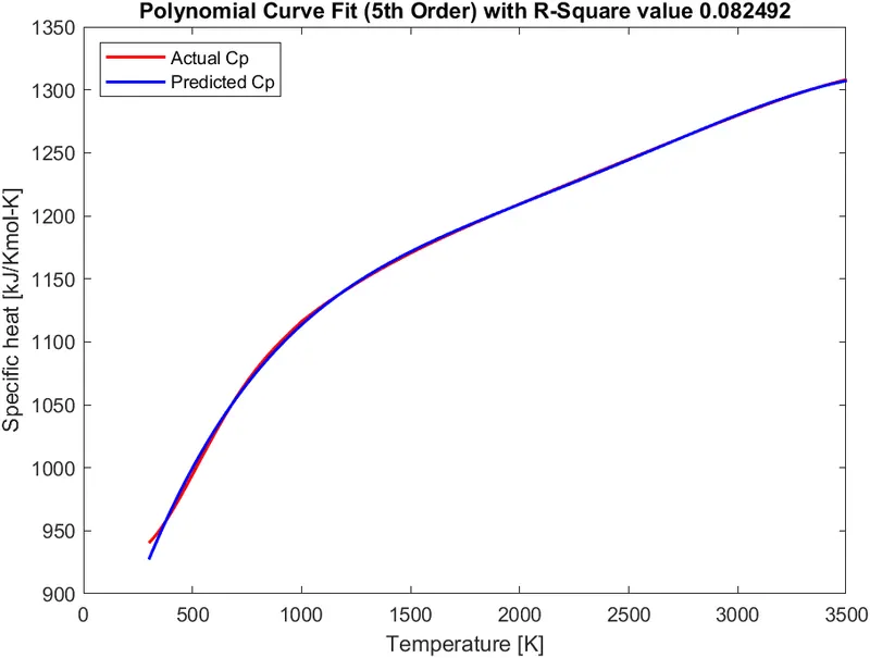
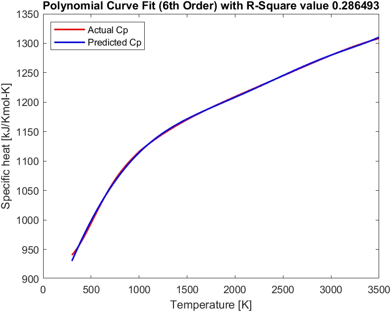
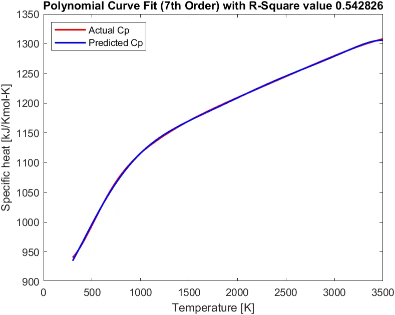
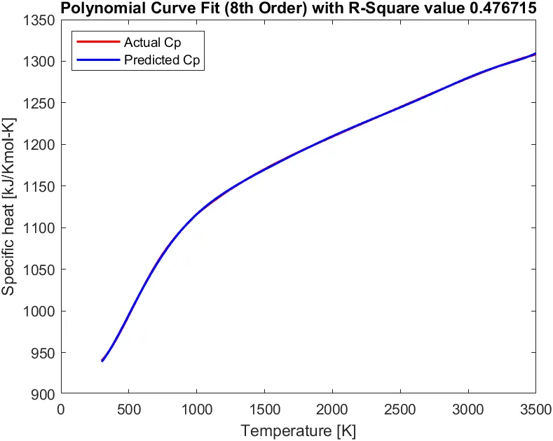
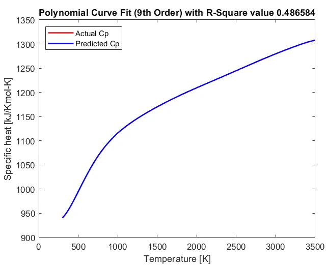
Outputs of further increasing Polynomial order
Results:
From the above plots we can observe that,
Visual Inspection - As the order of polynomial curve fit is increasing, Predicted Cp is getting more accurate.
R-Square Parameter - As the order of polynomial is increasing, goodness of fit is not in acceptable range.
Here, in linear curve fit though it is having the acceptable range of R-Square value we can say it is not a good fit by visual inspection of plot. This type of condition is called underfit (i.e. Underfit - If the order is too low to capture obvious trends in the data).
This is the reason it was mentioned in the above section of this article that visual examination is the foremost step for evaluating goodness of fit proceeding with statistical parameters.
Apart from this, we are getting a warning from Matlab stating Polynomial is badly conditioned if we use the polynomial order greater than or equals to 3 as shown in the below picture

Reason for this warning:
polyfit uses `X` to form Vandermonde matrix `V` with `n+1` columns and `m=`length() rows, resulting in the linear system
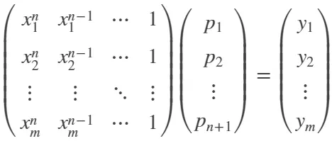
which polyfit solves with p = Vy. Since the columns in the Vandermonde matrix are powers of the vector x, the condition number of V is often large for high-order fits, resulting in a singular coefficient matrix. In those cases centering and scaling can improve the numerical properties of the system to produce a more reliable fit. This centering and scaling transformation improves the numerical properties of both the polynomial and the fitting algorithm.
centering and scaling transformation is done by just adding s,mu in polyfit & polyval commands as shown below
[coeff,s,mu] = polyfit(temp_step,cp_step,n)
new_cp = polyval(coeff,temp_step,s,mu)
This returns a structure S that can be used as an input to polyval to obtain error estimates and also returns mu, which is a two-element vector with centering and scaling values. mu(1) is mean(x), and mu(2) is std(x). Using these values, polyfit centers x at zero and scales it to have unit standard deviation, This centering and scaling transformation improves the numerical properties of both the polynomial and the fitting algorithm.
Let us try Matlab code to fit a cubic polynomial for the Cp data using Centering and Scaling:
%--------------------------------------------------------------------------------
clear all
close all
clc

data = load('data');                %Loading the data from the file

temp = data(:,1);                   %Retriving Temperature data
Cp = data(:,2);                     %Retriving Cp data

%Curve fitting is done by using Split-wise method
start = 0;                          %Assigining dummy value for starting step
stop = 0;                           %Assigining dummy value for ending step
predicted_Cp=zeros(length(Cp),1);   %Assigining dummy values for Cp to be predicted
frequency = 3200;                   %Frequency of steps
n = 3;                              %Order of polynomial

for i = 1:length(Cp)/frequency

start = stop+1;                     %Assigining the value for starting step
stop = stop + frequency;            %Assigining the value for ending step

temp_step = temp(start:stop);       %Loading the values of temperature in between the range
cp_step = Cp(start:stop);           %Loading the values of Cp in between the range

[coeff,s,mu] = polyfit(temp_step,cp_step,n); %To find the coeeficients
new_cp = polyval(coeff,temp_step,s,mu);    %To find the value of Predicted Cp

%To merge all the values of predicted Cp in one matrix
predicted_Cp(start:stop) = predicted_Cp(start:stop)+ new_cp;

end

%To check the goodness of fit
SSR = sum(predicted_Cp - mean(Cp))^2;
SSE = sum(Cp - predicted_Cp)^2;
SST = SSR + SSE;
R2 = SSR/SST

figure(1)
plot(temp,Cp,'r','linewidth',1.5)
hold on
plot(temp,predicted_Cp,'b','linewidth',1.5)
xlabel('Temperature [K]')
ylabel('Specific heat [kJ/Kmol-K]')
legend('Actual Cp','Predicted Cp','location','northwest')
title(sprintf('Cubic Polynomial Curve Fit (3rd Order) with R-Square value %f',R2))
%--------------------------------------------------------------------------------
Output:
No warning indications in command window
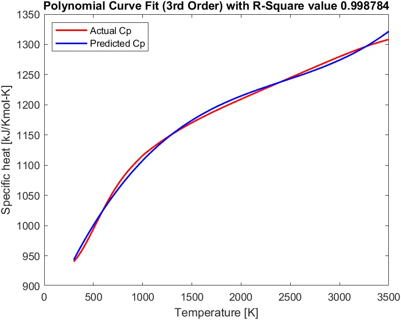
Outputs of further increasing Polynomial order with centering and scaling transformation
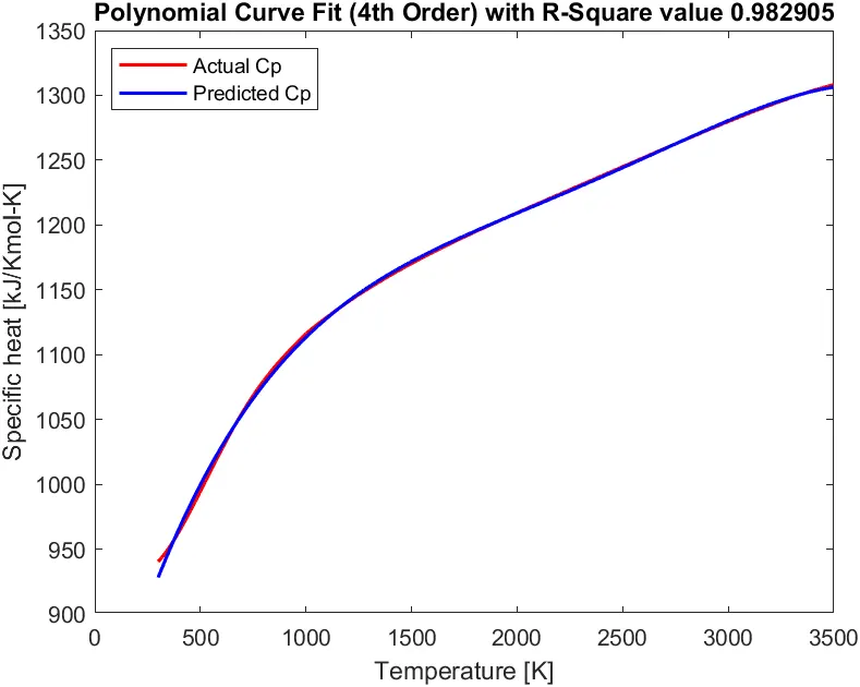
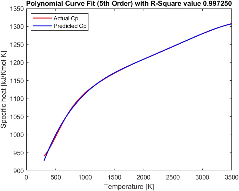
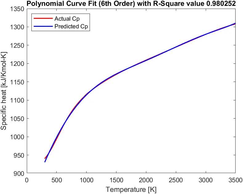
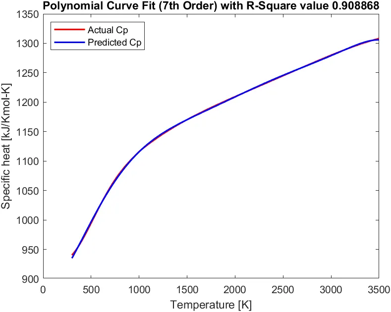
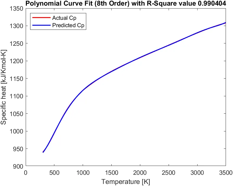
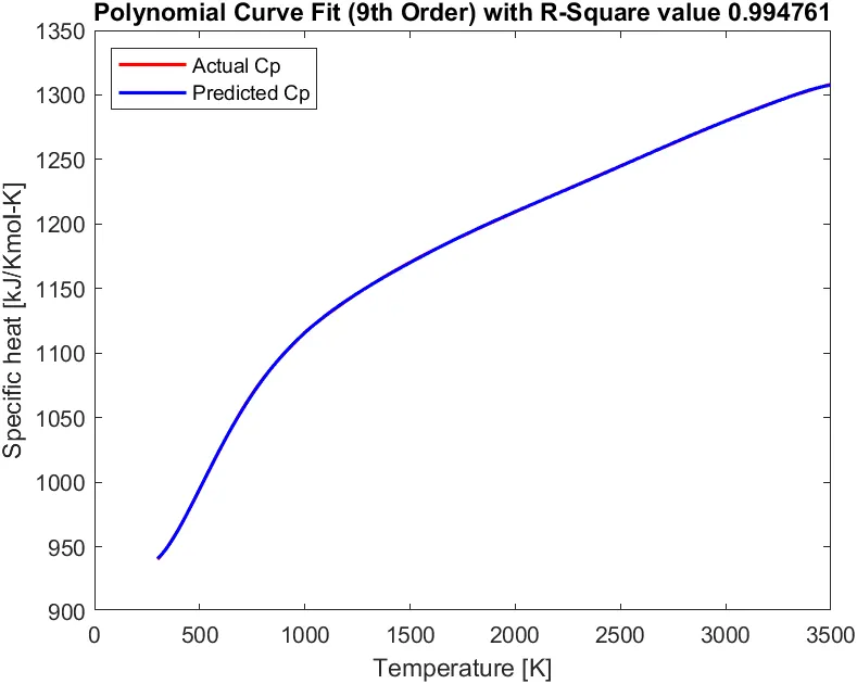
Results:
From the above plots we can observe that,
As the order of polynomial is increasing, Predicted Cp is getting more accurate with in the acceptable range of R-square value which says that the predicted Cp curve is a good fit.
However, increasing the degree of the polynomial fit using polyfit does not always result in a better fit. High-order polynomials can be oscillatory between the data points, leading to a poorer fit to the data. In those cases, we might use a low-order polynomial fit (which tends to be smoother between points) or a different technique, depending on the problem.
In this project we are going to look at the Split-wise method in which we are splitting the data into number of folds so that we can get a better fit with less order of polynomial.
Matlab code to fit the Cp data using split-wise method:
Order of polynomial n = 2
Frequency of steps = 400 i.e. we are dividing the given data (3200 data points) with 400 so that we get 8 sets with 400 data points in each.
%--------------------------------------------------------------------------------
clear all
close all
clc

data = load('data');                %Loading the data from the file

temp = data(:,1);                   %Retriving Temperature data
Cp = data(:,2);                     %Retriving Cp data

%Curve fitting is done by using Split-wise method
start = 0;                          %Assigining dummy value for starting step
stop = 0;                           %Assigining dummy value for ending step
predicted_Cp=zeros(length(Cp),1);   %Assigining dummy values for Cp to be predicted
frequency = 400;                    %Frequency of steps
n = 2;                              %Order of polynomial

for i = 1:length(Cp)/frequency

start = stop+1;                     %Assigining the value for starting step
stop = stop + frequency;            %Assigining the value for ending step

temp_step = temp(start:stop);       %Loading the values of temperature in between the range
cp_step = Cp(start:stop);           %Loading the values of Cp in between the range

[coeff] = polyfit(temp_step,cp_step,n); %To find the coeeficients
new_cp = polyval(coeff,temp_step);    %To find the value of Predicted Cp

%To merge all the values of predicted Cp in one matrix
predicted_Cp(start:stop) = predicted_Cp(start:stop)+ new_cp;

end

%To check the goodness of fit
SSR = sum(predicted_Cp - mean(Cp))^2;
SSE = sum(Cp - predicted_Cp)^2;
SST = SSR + SSE;
R2 = SSR/SST

figure(1)
plot(temp,Cp,'r','linewidth',1.5)
hold on
plot(temp,predicted_Cp,'b','linewidth',1.5)
xlabel('Temperature [K]')
ylabel('Specific heat [kJ/Kmol-K]')
legend('Actual Cp','Predicted Cp','location','northwest')
title(sprintf('Curve Fit (%dnd Order) with R-Square value %f',n,R2))
%--------------------------------------------------------------------------------
Output:
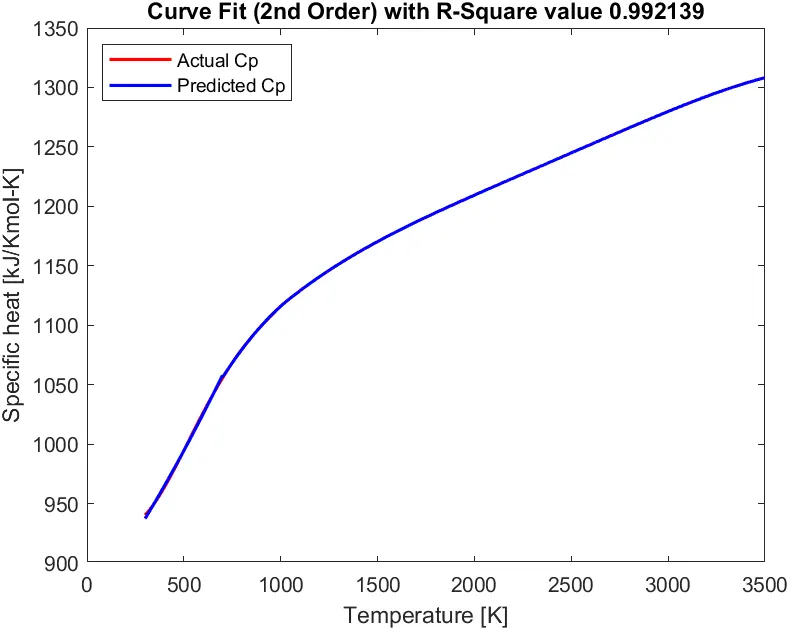
if we use
Order of polynomial n = 1 & Frequency of steps = 200
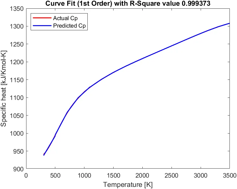
Order of polynomial n = 1 & Frequency of steps = 100
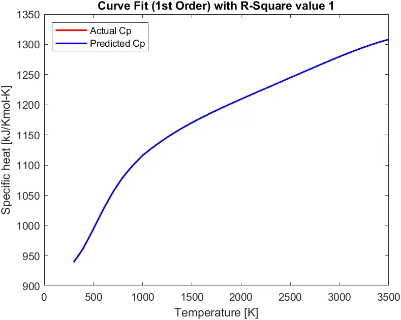
Conclusion:
1. Inorder to get the best fit we can undergo
i. Using higher degree of polynomial fit by obtaining error estimates and improving the numerical properties.
This can be done upto to a certain limit of order or else it may lead to Overfit (i.e. over-doing the requirement for the fit to ‘match’ the data trend-order too high)
ii. By reducing the data points using different methods like Split-wise method.
2. Split wise method along with centering and scaling can be used to improve the cubic fit.
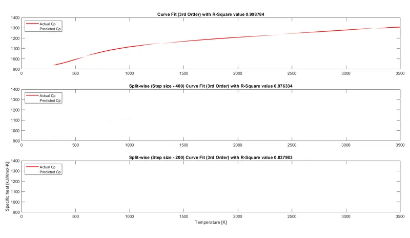
Red color in the plots represent the error between predicted curve and the given data. That means the fit is improved in case of split-wise method.
If we observe the plot, when step size = 200, R-square value is decresed this is due to overfit.
3. Using split-wise method we can get the perfect fit with appropriate degree of polynomial as shown in previous plot.