Rankine cycle Simulator
Objective:
- To Create a Rankine Cycle Simulator and to calculate the state points of the Rankine Cycle
- To plot the corresponding T-s and h-s plots for the chosen set of inputs
- To calculate some of its output parameters
Description:
The Rankine cycle is the basis of all large steam power plants. Steam based Rankine cycles are responsible for the majority of electric power generation in the world today. In coal-fired power plants, high-temperature, high-pressure steam is produced by converting the chemical energy stored in the coal into thermal energy and transferring the energy to the working fluid (e.g., water), which passes through the boiler to produce the steam. The steam from the boiler is expanded in a series of high- and low-pressure steam turbines, which convert the energy into mechanical shaft work to drive an electric generator and to produce electricity. After the last turbine stage, the steam is routed to a condenser, and the condensate is then pumped back into the boiler, repeating the cycle.
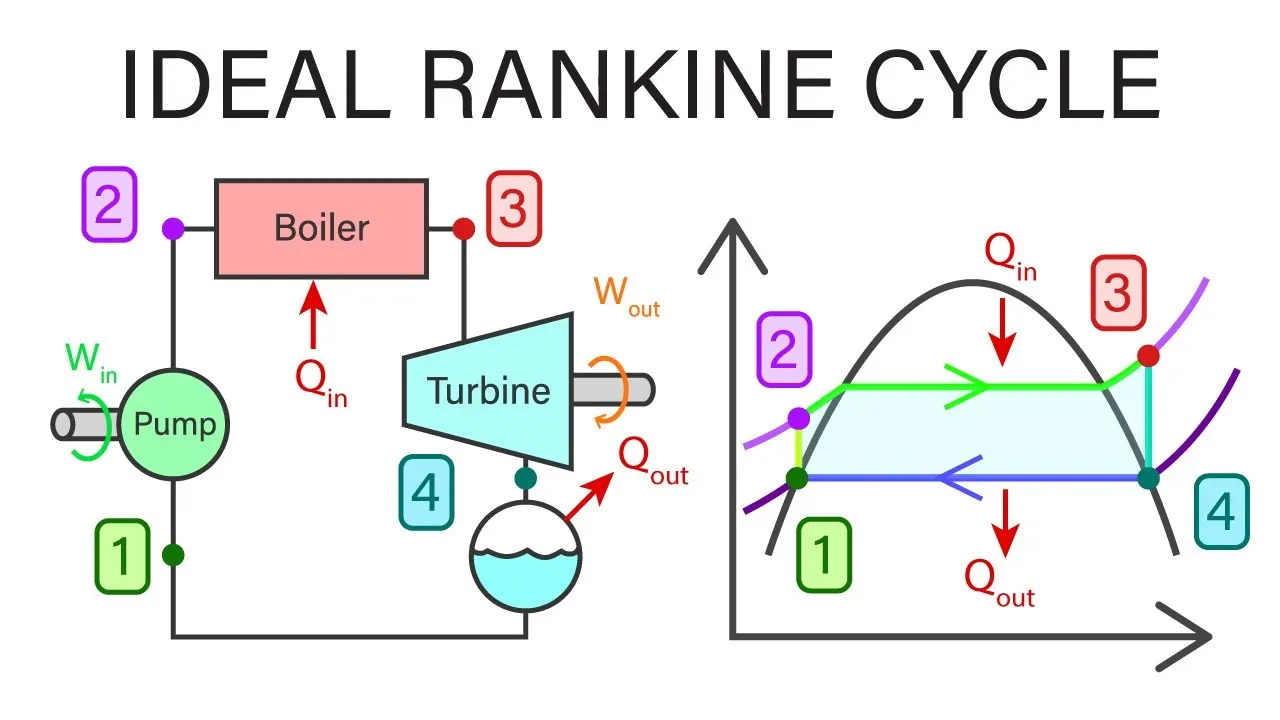
There are variations of the Rankine cycle, but for our project the basic Rankine cycle will be simulated for simplicity. The Rankine cycle is shown below.
Working Process of cycle:
A Rankine cycle in its simplest form consists of four processes carried out in a closed loop
The working fluid is compressed from low to high pressure (Step 1-2). At this stage, the pump requires little input energy because the fluid is a liquid.
The high-pressure liquid enters a boiler, where it is heated at constant pressure to the compressed liquid (Step 2-3) and two-phase (i.e., water and steam) mixture.
The steam is then expanded through a turbine to generate power (Step 3-4).
The expanded vapor, which is decreased in temperature and pressure, enters a condenser, where it is condensed at a constant pressure and temperature to become a saturated liquid and the unavailable heat is rejected to the atmospheric sink (Step 4-1).
Net workdone `W_(Net) = W_(t) - W_p`
Thermal efficiency `eta = (Q_i - Q_o)/Q_i`
Back work ratio = `= W_p/W_t;`
Specific Steam Consumption `= 3600/W_(Net)`
Matlab code with explaonation;
clear all
close all
clc
%%Showing the Process of Rankine cycle
disp(sprintf('ttRankine cycle simulatorn'))
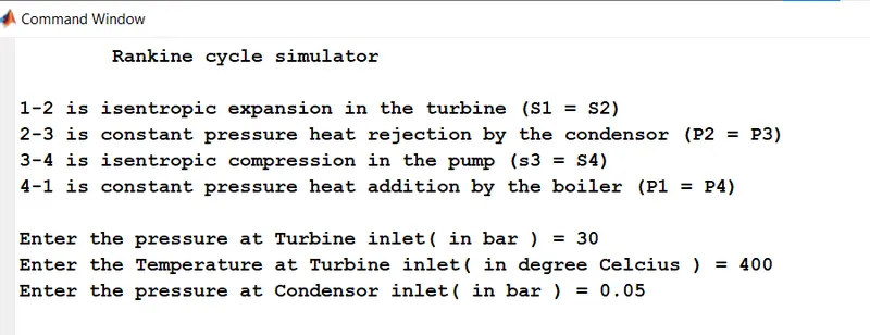
disp('1-2 is isentropic expansion in the turbine (S1 = S2)')
disp('2-3 is constant pressure heat rejection by the condensor (P2 = P3)')
disp('3-4 is isentropic compression in the pump (s3 = S4)')
disp('4-1 is constant pressure heat addition by the boiler (P1 = P4)')
disp('   ')

%% Taking inputs to create a Rankine cycle
%To Enter Turbine inlet Pressure
P1 = input('Enter the pressure at Turbine inlet( in bar ) = ');
%To Enter Turbine inlet temperature
T1 = input('Enter the Temperature at Turbine inlet( in degree Celcius ) = ');
%To Enter Condensor Pressure
P3 = input('Enter the pressure at Condensor inlet( in bar ) = ');

%% Extracting S1 and H1 from data file - Saturated Region
h1 = XSteam('h_pT',P1,T1);
s1 = XSteam('s_pT',P1,T1);

%% As per Rankine Cycle conditions
P2 = P3;
P4 = P1;
s2 = s1;

%% Extracting T2, S2 and H2 from data file using Dryness fraction - Mixed Region
sf_2 = XSteam('sL_P',P2);
sg_2 = XSteam('sV_P',P2);
sfg_2 = (sg_2-sf_2);

%Dryness fraction can be calculated as shown s = sf + x*sfg    %x  = (s-sf)/sfg
X = (s2-sf_2)/sfg_2;

hf_2 = XSteam('hL_P',P2);
hfg_2 = (XSteam('hV_P',P2) - hf_2);
h2 = hf_2 + X*hfg_2;
T2 = XSteam('Tsat_p',P2);

%% Extracting T3, S3 and H3 from data file - Liquid Region
h3 = XSteam('hL_P',P3);
s3 = XSteam('sL_P',P3);
T3 = T2;

%% Extracting T4, S4 and H4 from data file - Liquid Region
h4 = h3+ XSteam('vL_P',P2)*(P1-P2)*100;
s4 = s3;
cp4 = XSteam('Cp_ps',P4,s4);
cv4 = XSteam('Cv_ps',P4,s4);
k = cp4/cv4;
T4 = T3/(P3/P4)^((k-1)/k);

%% Calculating the cycle parameters
W_t = h1-h2;                 % Workdone by Turbine
W_p = h4-h3;                 % Workdone by Pump
W_net = W_t - W_p;           % Total Workdone
B_WR = W_p/W_t;              % Back Work ratio
Q_in = h1-h4;                % Heat Inlet
Q_out = h2-h3;               % Heat outlet
Th_eff = (Q_in-Q_out)/Q_in;  % Thermal efficiency
SSC = 3600/W_net;            % Specific Steam Consumption

%% Displaying the calculated parameters

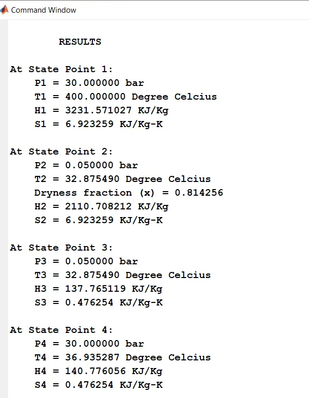
disp(sprintf('nttRESULTS'))
disp(sprintf('nAt State Point 1:'))
disp(sprintf('tP1 = %f bar',P1))
disp(sprintf('tT1 = %f Degree Celcius',T1))
disp(sprintf('tH1 = %f KJ/Kg',h1))
disp(sprintf('tS1 = %f KJ/Kg-K',s1))


disp(sprintf('nAt State Point 2:'))
disp(sprintf('tP2 = %f bar',P2))
disp(sprintf('tT2 = %f Degree Celcius',T2))
disp(sprintf('tDryness fraction (x) = %f',X))
disp(sprintf('tH2 = %f KJ/Kg',h2))
disp(sprintf('tS2 = %f KJ/Kg-K',s2))

disp(sprintf('nAt State Point 3:'))
disp(sprintf('tP3 = %f bar',P3))
disp(sprintf('tT3 = %f Degree Celcius',T3))
disp(sprintf('tH3 = %f KJ/Kg',h3))
disp(sprintf('tS3 = %f KJ/Kg-K',s3))

disp(sprintf('nAt State Point 4:'))
disp(sprintf('tP4 = %f bar',P4))
disp(sprintf('tT4 = %f Degree Celcius',T4))
disp(sprintf('tH4 = %f KJ/Kg',h4))
disp(sprintf('tS4 = %f KJ/Kg-K',s4))

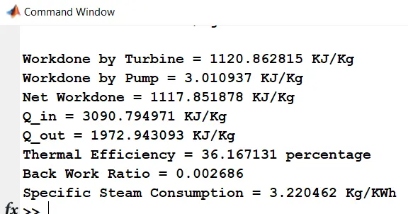
disp(sprintf('nWorkdone by Turbine = %f KJ/Kg',W_t))
disp(sprintf('Workdone by Pump = %f KJ/Kg',W_p))
disp(sprintf('Net Workdone = %f KJ/Kg',W_net))
disp(sprintf('Q_in = %f KJ/Kg',Q_in))
disp(sprintf('Q_out = %f KJ/Kg',Q_out))
disp(sprintf('Thermal Efficiency = %f percentage',Th_eff*100))
disp(sprintf('Back Work Ratio = %f',B_WR))
disp(sprintf('Specific Steam Consumption = %f Kg/KWh',SSC))

%% To create a vapour dome w.r.t T-S
T = 1:0.01:500;
for i = 1:length(T)
    sf(i) = XSteam('sL_T',T(i));
    sg(i) = XSteam('sV_T',T(i));
end

sg_1 = XSteam('sV_P',P1);
Tg_1 = XSteam('Tsat_p',P1);
sl_1 = XSteam('sL_T',Tg_1);
count = 0;
for i = length(T):-1:1
    if count < 1
    if sf(i) > 0.1
      critial_point_location = i;
      count = count + 1;
    end
    end
end
%to find critical point
Y_coordinate = T(critial_point_location);
X_coordinate = (max(sf)+ min(sg))/2;


%% Ploting Vapour dome along with critical point
figure(1)
plot(sf,T,'b','linewidth',1.25)
hold on
plot(sg,T,'r','linewidth',1.25)
plot(X_coordinate,Y_coordinate,'*k','linewidth',1)
xline(X_coordinate,'--g','linewidth',1)
yline(Y_coordinate,'--g','linewidth',1)


%% To create a vapour dome w.r.t H-S
for i = 1:length(T)
    hf(i) = XSteam('hL_T',T(i));
    hg(i) = XSteam('hV_T',T(i));
end
%to find critical point
Y_cordinate = (max(hg));
[Y_cordinate,idy] = (max(hg));
X_cordinate = sg(idy);

%% Ploting vapour dome along with critical point
figure(2)
plot(sf,hf,'b','linewidth',1.25)
hold on
plot(sg,hg,'r','linewidth',1.25)
plot(X_cordinate,Y_cordinate,'*k','linewidth',1)
xline(X_cordinate,'--g','linewidth',1.25)
yline(Y_cordinate,'--g','linewidth',1.25)


%% Ploting cycle : T-S plot
fh = figure(1);
fh.WindowState = 'maximized';
plot ([s1,s2,s3,s4,sl_1,sg_1,s1],[T1,T2,T3,T4,Tg_1,Tg_1,T1],'k','linewidth',1.25)
text(s1+0.1,T1,'1')
text(s2+0.1,T2,'2')
text(s3-0.2,T3,'3')
text(s4-0.2,T4+10,'4')
text(sl_1-0.3,Tg_1,"4'")
text(sg_1-0.1,Tg_1-10,"1'")
axis([0 10 0 450])
xlabel('Entropy (S)');
ylabel('Temperature (T)');
legend('Liquid region','Vapour Region','Critical point','Critical point x-line','Critical point y-line','Cycle')
tittle = {'Rankine Cycle','T - S Plot'};
title([tittle],'FontName','Lucida Console');

%% Ploting cycle : H-S plot
fh = figure(2);
fh.WindowState = 'maximized';
plot ([s1,s2,s3,s4,s1],[h1,h2,h3,h4,h1],'k','linewidth',1.25)
text(s1+0.1,h1,'1')
text(s2+0.1,h2,'2')
text(s3-0.2,h3,'3')
text(s4-0.2,h3,'4')
xlabel('Entropy (S)');
ylabel('Enthalpy (H)');
legend('Liquid region','Vapour Region','Critical point','Critical point x-line','Critical point y-line','Cycle')
tittle = {'Rankine Cycle','H - S Plot'};
title([tittle],'FontName','Lucida Console');
Output:
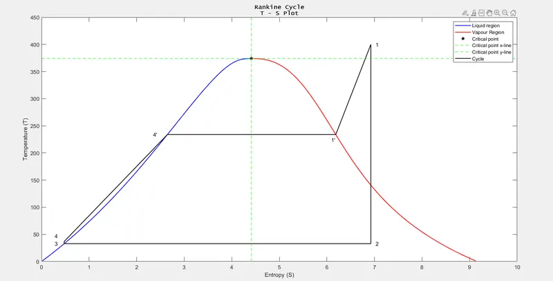
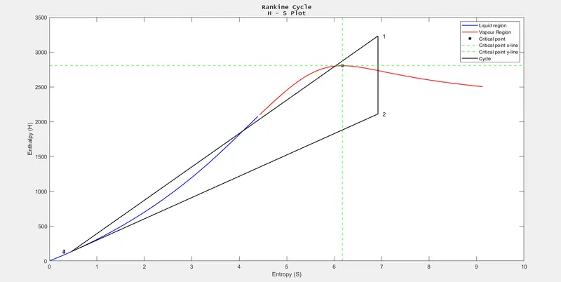
Note:
Here, the values required from steam table are acheived from the XSTEAM matlab file