Solving of linear systems using iterative methods
Objective: To solve eigen values and spectral radius for a matrix Ax=B using iterative solvers
To find the effect of spectral radius on solution
Basics of matrices:
A vector which satisfies Ax = λx for some number λ is called an eigenvector of the matrix M and λ is called the eigenvalue of A corresponding to x. (x is called an eigenvector corresponding to λ.)
The condition Ax = λx can be rewritten as (A- λI) v = 0. This equation says that the matrix (A- λI) takes x into the 0 vector, which implies that (M - xI) cannot have an inverse so that its determinant must be 0.
The equation det (A- λI) = 0 is a polynomial equation in the variable λ for given A. It is called the characteristic equation of the matrix A. You can solve it to find the eigenvalues λ, of A.
In a simple way eigen values are the roots of the equation and spectral radius is the highest value of eigen values denoted by ϱ(rho)
Once you know an eigenvalue λ of A, there is an easy way to find a column eigenvector corresponding to λ (which works when λ is not a multiple root of the characteristic equation).
Solving linear systems:
The most basic problem in linear algebra: solving the linear algebraic system Ax = B, consisting of n equations in n unknowns. We assume that the coefficient matrix A is non-singular, and so the solution x = A−IB is unique.
We will introduce popular iterative methods that can be used to approximate the solution for certain classes of coefficient matrices. The resulting algorithms will provide an attractive alternative to Gaussian Elimination, particularly when dealing with the large, sparse systems that arise in the numerical solution to differential equations. One major advantage of an iterative technique is that it (typically) produces progressively more and more accurate approximations to the solution, and hence, by prolonging the iterations, can, at least in principle, compute the solution to any desired order of accuracy. Moreover, even performing just a few iterations may produce a reasonable approximation to the true solution — in stark contrast to Gaussian Elimination, where one must continue the algorithm through to the bitter end before any useful information can be extracted. A partially completed Gaussian Elimination is of scant use! A significant weakness is that iterative schemes are not universally applicable, and their design relies upon the detailed structure of the coefficient matrix.
The three most important iterative schemes used to accurately approximate the solutions to linear algebraic systems. The classical Jacobi method is the simplest, while an evident serialization leads to the popular Gauss–Seidel method. Completely general convergence criteria are hard to formulate, although convergence is assured for the important class of diagonally dominant matrices that arise in many applications. A simple modification of the Gauss–Seidel scheme, known as Successive Over-Relaxation (SOR), can dramatically speed up the convergence rate, and is the method of choice in many modern applications.
Stationary iterative methods solve a linear system with an operator approximating the original one; and based on a measurement of the error in the result (the residual), form a "correction equation" for which this process is repeated. While these methods are simple to derive, implement, and analyse, convergence is only guaranteed for a limited class of matrices.
In a simple way iterative methods are used to find the eigen values of the linear system Ax=B but each iterative method consists its own iterative matrix to find the eigen values.
Let us consider a matrix Ax=B
`ubrace{[[5,1,2],[-3,9,4],[1,2,-7]]}_{[A]} ubrace{[[x_1],[x_2],[x_3]]}_{[X]} = ubrace{[[10],[-14],[33]]}_{[B]}`
Where, A is the coefficient matrix
B is the residual matrix
x is the unknown matrix to be found
To find the roots using iterative solvers any matrix Ax=B is splitted into the form of `A = D + U + L`
`ubrace{[[5,1,2],[-3,9,4],[1,2,-7]]}_{[A]}= ubrace{[[5,0,0],[0,9,0],[0,0,-7]]}_{[D]} + ubrace{[[0,1,2],[0,0,4],[0,0,0]]}_{[U]}+ ubrace{[[0,0,0],[-3,0,0],[1,2,0]]}_{[L]}`
Where, D is diagonal matrix
U is upper triangular matrix
L is lower triangular matrix
using these splitted matrices required iterative matrices are found according to the method
Iterative matrix used in Jacobi method
`D^-1(L+U)`
Iterative matrix used in Gauss-seidel method
`U* (L+D)^-1`
Iterative matrix used in SOR method
`(D+omega*L)^-1*(omega*U-(1-omega)*D)`
ω is the relaxation factor
Spectral radius (ρ):
The spectral radius of a matrix T is defined as the maximal modulus of all of its real and complex eigenvalues: ρ(T) = max { | λ1|, . . ., | λk| }.
Conditions for convergence:
1. The convergence of a linear iterative system is governed by the spectral radius or
largest eigenvalue (in modulus) of the coefficient matrix.
A matrix is convergent if and only if its spectral radius is strictly less than one: ρ(T) < 1.
The spectral radius prescribes the rate of convergence of the solutions to equilibrium. The smaller the spectral radius, the faster the solutions go to 0.
2. If A is strictly diagonally dominant, then the associated iteration scheme converges.
Main Matlab code :
close all
clear all
clc

%%considering a linear matrix Ax=B
A=[5 1 2 ; -3 9 4; 1 2 -7];
%X=[x1;x2;x3];
B=[10;-14;33];
eigen=eig(A);
spectral_radius=max(abs(eigen));

%to split the matrix A into D,L,U
D=diag(diag(A));       %to create a diagonal matrix
L=tril(A)-D;           %to create lower triangular matrix
U=triu(A)-D;           %to create upper triangular matrix

k= [0.08869:0.01:1 1];                %magnification_factor
for i = 1: length(k)
    %%jacobi method
    [iter_j,x_j,spectral_radius_j,eigen_j]=jacobi_iteration(B,L,D,U,k(i));

    if any(isnan(x_j), 'all')
    figure(1)
    plot(k(i),spectral_radius_j, '-or','linewidth',2)
    yline(1,'-k')
    hold on

    figure(2)
    plot(spectral_radius_j,iter_j, '-or','linewidth',2)
    hold on
    set(gca, 'XDir','reverse')
    else
    figure(1)
    plot(k(i),spectral_radius_j, '-ob','linewidth',2)
    figure(2)
    plot(spectral_radius_j,iter_j, '-ob','linewidth',2)
    grid on
    set(gca, 'XDir','reverse')
    end

     %% Gauss-seidel method
    [iter_gs,x_gs,spectral_radius_gs,eigen_gs]=gauss_seidel_iteration(B,L,D,U,k(i));

    if any(isnan(x_gs), 'all')
    figure(3)
    plot(k(i),spectral_radius_gs, '-or','linewidth',2)
    yline(1,'-k')
    hold on

    figure(4)
    plot(spectral_radius_gs,iter_gs, '-or','linewidth',2)
    hold on
    set(gca, 'XDir','reverse')
    else
    figure(3)
    plot(k(i),spectral_radius_gs, '-ob','linewidth',2)
    figure(4)
    plot(spectral_radius_gs,iter_gs, '-ob','linewidth',2)
    grid on
    set(gca, 'XDir','reverse')
    end

    %% SOR method
    [iter_SOR,x_SOR,spectral_radius_SOR,eigen_SOR]=SOR_iteration(B,L,D,U,k(i));

    if any(isnan(x_SOR), 'all')
    figure(5)
    plot(k(i),spectral_radius_SOR, '-or','linewidth',2)
    yline(1,'-k')
    hold on

    figure(6)
    plot(spectral_radius_SOR,iter_SOR, '-or','linewidth',2)
    hold on
    set(gca, 'XDir','reverse')
    else
    figure(5)
    plot(k(i),spectral_radius_SOR, '-ob','linewidth',2)
    figure(6)
    plot(spectral_radius_SOR,iter_SOR, '-ob','linewidth',2)
    grid on
    set(gca, 'XDir','reverse')
    end

    %% optional code

    %to find the output matrix using inbuilt functions
    A1 = L + U + k(i)*D;
    X_direct = A1^-1*B
    % conditions for diagonal dominance
    dd1 = abs(A1(4))+ abs(A1(7));
    dd2 = abs(A1(2))+ abs(A1(8));
    dd3 = abs(A1(3))+ abs(A1(6));

    % to display magnification number
    At_magnification_factor_k = k(i)

    % to display dominance condition at every K value
     if dd1 < abs(A1(1)) & dd2 < abs(A1(5)) & dd3 < abs(A1(9))
         disp('The matrix A is diagonally dominant')
     else
         disp('The matrix A is diagonally not dominant')
     end
    spectral_radius_using___Jacobi___Gauss___SOR = [spectral_radius_j,spectral_radius_gs,spectral_radius_SOR]
%     Note: 1st column -   X matrix using jacobi method
%           2nd column -   X matrix using seidel method
%           3nd column -   X matrix using SOR method
    X_matrix_using___Direct___Jacobi___Gauss___SOR = [X_direct,x_j,x_gs,x_SOR]
%     Note: 1st column  -   X matrix using direct solving method using matlab inbuilt functions
%           2nd column -   X matrix using jacobi method
%           3rd column -   X matrix using seidel method
%           4th column -   X matrix using SOR method

    number_of_iterations___Jacobi___Gauss___SOR  = [iter_j,iter_gs,iter_SOR]
%     Note: 1st column -   X matrix using jacobi method
%           2nd column -   X matrix using seidel method
%           3nd column -   X matrix using SOR method
end

figure(1)
xlabel('Magnification factor (k)')
ylabel('Spectral radius')
title('Magnification factor vs Spectral radius using Jacobi method')

figure(3)
xlabel('Magnification factor (k)')
ylabel('Spectral radius')

title('Magnification factor vs Spectral radius using Gauss method')

figure(5)
xlabel('Magnification factor (k)')
ylabel('Spectral radius')
title('Magnification factor vs Spectral radius using SOR method')

figure(2)
xlabel('Spectral radius')
ylabel('number of iterartions')
title('Spectral radius vs number of iterations using Jacobi method')

figure(4)
xlabel('Spectral radius')
ylabel('number of iterartions')
title('Spectral radius vs number of iterations using Gauss method')

figure(6)
xlabel('Spectral radius')
ylabel('number of iterartions')
title('Spectral radius vs number of iterations using SOR method')
Jacobi function code
function [iter_j,x_j,spectral_radius_j,eigen_j]=jacobi_iteration(B,L,D,U,k)

error = 9e9;
tolerance = 1e-6;
D=k*D;              %to multiply magnification factor with diagonal matrix
jacobi_iterative_matrix = inv(D)*(L+U);
x_old = [0;0;0];
iter_j = 1;
 while error>tolerance
     x_j = (inv(D)*B) - (jacobi_iterative_matrix * x_old);
     error = max(abs(x_j-x_old));
     x_old=x_j;
     iter_j = iter_j + 1;
 end
 eigen_j=(roots(poly(jacobi_iterative_matrix)));
 spectral_radius_j=max(abs(eigen_j));
end
Gauss-seidel function code
function [iter_gs,x_gs,spectral_radius_gs,eigen_gs]=gauss_seidel_iteration(B,L,D,U,k)

error = 9e9;
tolerance = 1e-6;
D=k*D;              %to multiply magnification factor with diagonal matrix
gauss_iterative_matrix = inv(L+D)*U;
x_old = [0;0;0];
iter_gs = 1;
 while error>tolerance
     x_gs = (inv(L+D)*B) - (gauss_iterative_matrix * x_old);
     error = max(abs(x_gs-x_old));
     x_old=x_gs;
     iter_gs = iter_gs + 1;
 end
 eigen_gs=(roots(poly(gauss_iterative_matrix)));
 spectral_radius_gs=max(abs(eigen_gs));
end
SOR function code
function [iter_SOR,x_SOR,spectral_radius_SOR,eigen_SOR]=SOR_iteration(B,L,D,U,k)

tolerance = 1e-6;
o=0.4:0.1:1;        %relaxation factor omega
D=k*D;              %to multiply magnification factor with diagonal matrix

iter_SOR = 9e9;
for i=length(o):-1:1
    error = 9e9;
    sor_iterative_matrix =(inv(D+(o(i)*L)))*((o(i)*U)-((1-o(i))*D));
x_old = [0;0;0];
iter_SOR_new = 1;
 while error>tolerance
     x_SOR = (inv(D+(o(i)*L)))*(o(i)*B)-sor_iterative_matrix*x_old;
      error = max(abs(x_SOR-x_old));
     x_old=x_SOR;
     iter_SOR_new = iter_SOR_new + 1;
 end
 if any(isnan(x_SOR), 'all')
 iter_SOR = 9e9;
 end
 if iter_SOR<iter_SOR_new
     break;
 end
 iter_SOR = iter_SOR_new;
end
 eigen_SOR=(roots(poly(sor_iterative_matrix)));
 spectral_radius_SOR=max(abs(eigen_SOR));
 end
Output:
Note: 1st column - X matrix using direct solving method using matlab inbuilt functions
2nd column - X matrix using jacobi method
3nd column - X matrix using seidel method
4nd column - X matrix using SOR method
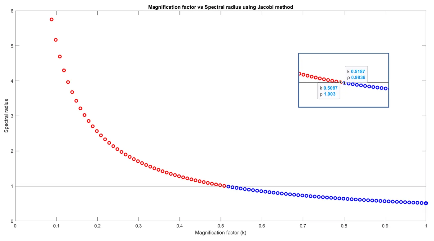
Plot 1 - Magnification factor vs Spectral radius - Jacobi method
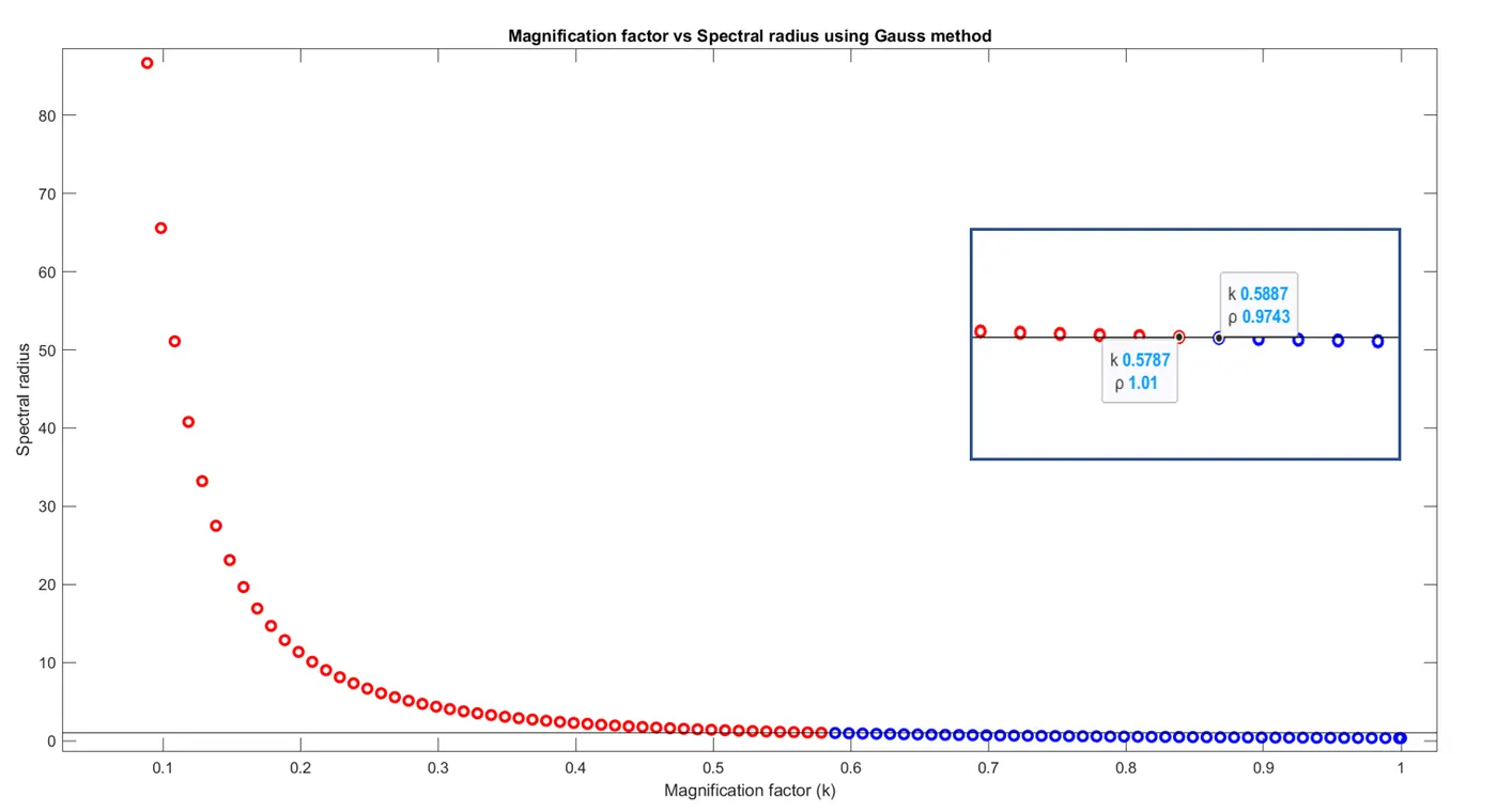
Plot 2 - Magnification factor vs Spectral radius - Gauss-seidel method
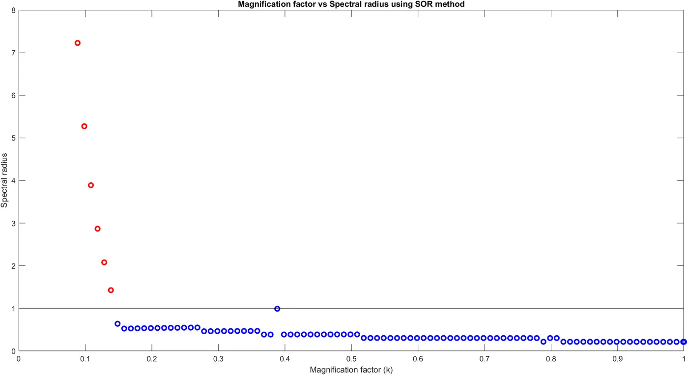
Plot 3 - Magnification factor vs Spectral radius - SOR method
From the above video we can observe that,
1. After a certain value of magnification factor (k), the iterative solvers like Jacobi, Gauss-seidel and SOR is giving the same result as that of direct solving method using matlab inbuilt functions.
2. Upto a certain value of k, output matrix is shown as NaN instead of numbers (i.e..there are no value). These are seen when the solution is not converged but after a certain value of k the output matrix is started showing numbers which says that the solution is converged and the output is obtained.
3. All the three iterative methods are not started converging from the same magnification factor.
From the above plots we can observe that,
1. In plot 1,2 & 3 - red circle shows the non convergence & blue circle shows the convergence of matrix A.
2. From plot 2 & 3 - the convergence took place only below the spectral radius value 1 as per our condition stated above. This shows us that the convergence of matrix is depending on the spectral radius.
In our case, the min value of k is 0.5887.
3. From plot 1 & 2 - convergence of solution is obtained from the lower value of k in Jacobi method comparing to Gauss-seidel method.
Jacobi is started from - 0.5187
Gauss-seidel is started from - 0.587
which means that there are some situations where jacobi is more reliable method.
4. From plot 3 - SOR method is converging earlier than jacobi and seidel method. This is because of multiplication of Relaxation parameter ω to seidel method. A single value of ω will not give the converged results in every case it should be choose accordingly. Correct value of ω will give the convergence with less number of iterations
Note: 1st column - using jacobi method
2nd column - using seidel method
3rd column - using SOR method
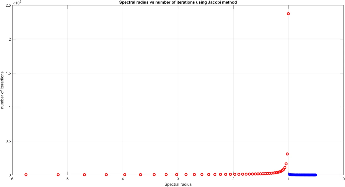
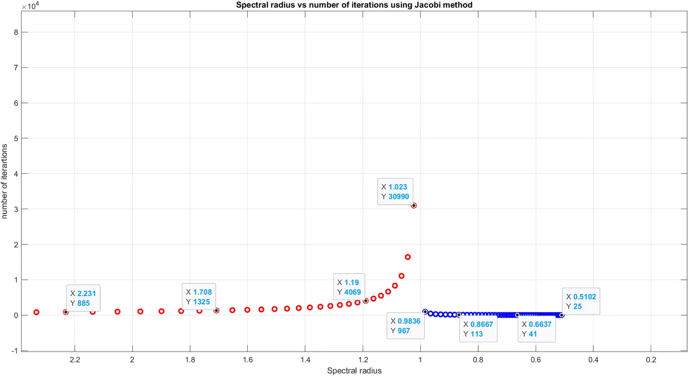
Plot 1 - Spectral radius vs Number of iterations - Jacobi method
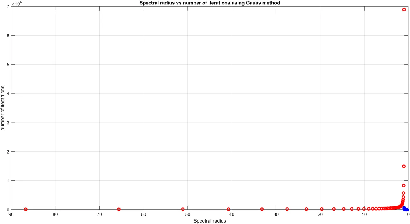
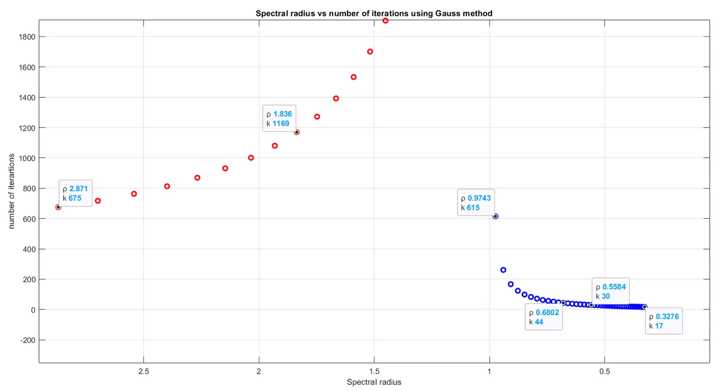
Plot 2 - Spectral radius vs Number of iterations - Gauss-seidel method
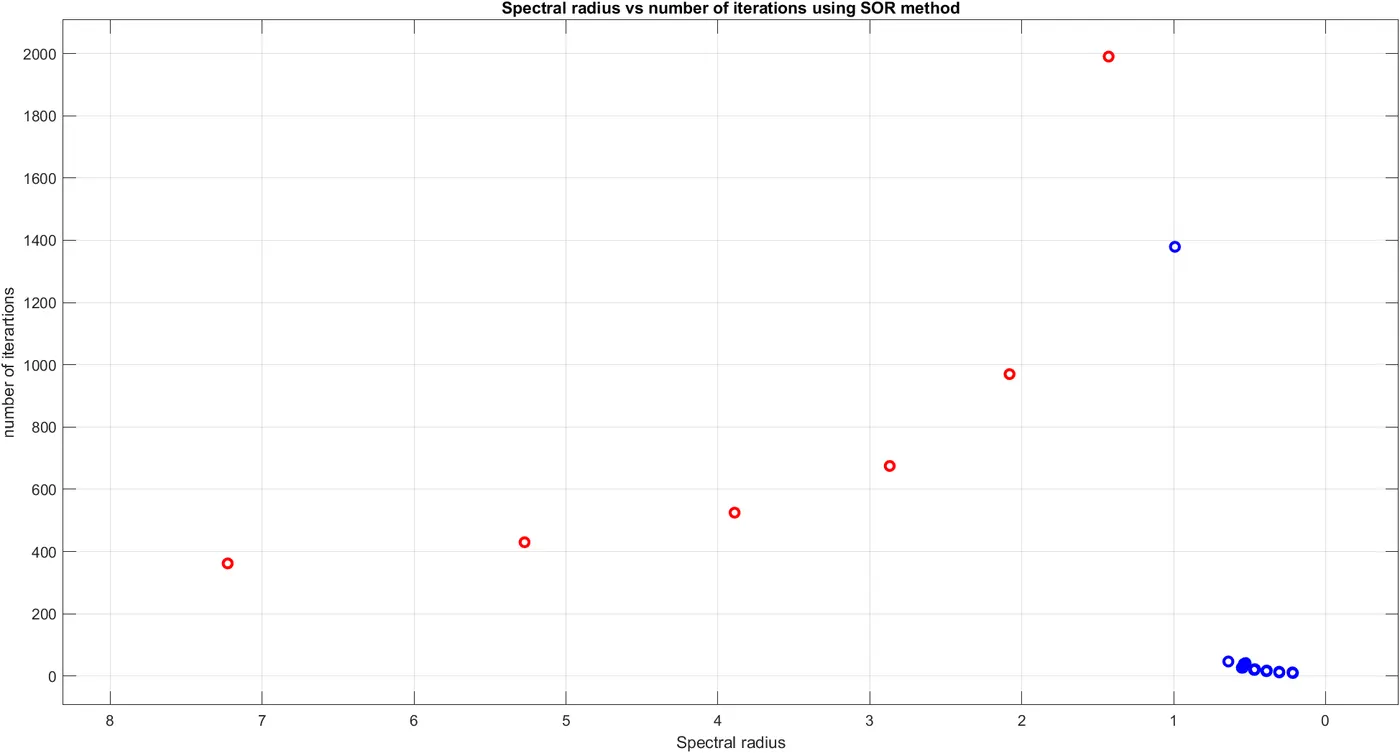
Plot 3 - Spectral radius vs Number of iterations - SOR method
From the above video we can observe that,
1. As the magnification factor is increasing, the spectral radius goes on decreasing.
2. After a certain value of magnification factor k, though the iterative solvers like Jacobi, Gauss-seidel and SOR is giving the same results but the number of iterations are different.
3. From the range of k value from 0.5887 to 0.6687, the number of iterations using jacobi method is less than the number of iterations obtained using Gauss-seidel method.
4. After the value of k from 0.6687 the number of iterations obtained using Gauss-seidel method is less than that of Jacobi method.
5. Number of iterations using SOR is always smaller than Gauss-seidel and Jacobi.
From the above plots we can observe that,
1. In plot 1,2 & 3 - red circle shows the non convergence & blue circle shows the convergence of matrix A.
2. From plot 1,2 & 3 - as the spectral radius is decreasing, the number of iterations are increasing in non-convergence region and after entering the convergence region there is a tremendious drop in number of iterations in all the three methods
Note: 1st column - using jacobi method
2nd column - using seidel method
3rd column - using SOR method
From the above video we can observe that,
1. The minimum value of k to satisfy the diagonal dominant condition is = 0.7787.
2. According to theory, the solution should be converged if the matrix is strictly a diagonal dominant. But, from k = 0.5187 though the matrix is not a diagonal dominant the solution is tending to converg using jacobi method and from k=0.5887 using seidel method.
Conclusion:
1. We encountered a situation where the Jacobi method converges faster than Gauss-seidel. This is an example which states that there are some situation where jacobi will converge faster and more reliable than Gauss-seidel.
2. But in many practical situations Gauss–Seidel tends to converge roughly twice as fast as Jacobi.
3. The solution is strictly converging when it is satisfying both the condtions
i. Spectral radius < 1 &
ii. coefficient matrix is strictly diagonal dominant.
4. In case of SOR method the rate of convergence is not only governed by the spectral radius of the matrix. Relaxation parameter ω plays a role to obtain the convergence. The goal is to choose the relaxation parameter ω so as to make the spectral radius of A as small as possible. As we will see, a clever choice of ω can result in a dramatic speed up in the convergence rate.
5. There are some situations where the solution is converged though it is not a diagonally dominant when the spectral radius is less than 1. This clearly shows us that apart from the above mentioned (3) conditions there are some criterias where the solution can be converged.
Reference: https://www-users.math.umn.edu/~olver/num_/lni.pdf