Simulation of Flow through a Axi-symmetry pipe in Open Foam and verifying Hagen Poiseuille law

Objective:

• To write a program in Matlab that can generate the computational mesh automatically for any wedge angle and grading schemes validating with the Hagen poiseuille's equation to check the fedility of the solution.
• Showing the fully developed velocity profile and Post processing the velocity and shear stress.

Abstract:

Hagen–Poiseuille flow (or simply Poiseuille flow) is applicable to a variety of applications ranging from macroscopic pipes in industries to the flow of blood in veins. This project presents the simulation of Hagen–Poiseuille Flow (Laminar-Incompressible Flow) through a pipe having constant circular cross-section throughout the length. The whole report can be divided into two sections:

The former part aims to implement automation in the generation of computational mesh file, time-control file, and other necessary script files (later, these will be used by OpenFOAM to run the simulation) using MATLAB. As the flow has axis-symmetrical nature, only a reduced model (Wedge) is considered instead of entire circular pipe, thus reducing computational efforts extensively. A suitable wedge angle is considered to simulate the flow realistically.

In the latter part, the CFD analysis is performed using an open-source CFD toolbox- OpenFOAM®, which utilized all the previously generated scripts files.

This project is principally focused to analyze the development of velocity profile in the Hydrodynamic Entrance Region and variation of shear stress along the axial direction of the pipe. During this project, obtained CFD data is validated with analytical values calculated from Hagen–Poiseuille equations, to assure the fidelity of the numerical results. Besides, this report includes the variation of velocity profile and pressure drop at different cross-sections throughout the length, and it also aimed to calculate the shear stress profiles as a part of post-processing results.

Geometry:

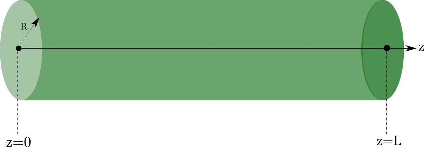
Consider an incompressible laminar and Newtonian flow through a pipe having constant circular cross-section throughout the length (or Hagen–Poiseuille flow). The basic model geometry is shown in the above figure. The diameter of the pipe `D = 0.03m` and length of pipe `L = 5m`, and water can be considered as the working fluid in the pipe.

As per the first part of analysis, writing a MATLAB code to generate the required computational files like blockMeshDict, controlDict, p, U etc.. which are later used by openFOAM to simulate the flow.

In the second part, set-up the physical model by utilizing previously generated script files and run the CFD simulation using openFOAM. Geometry, loadings, boundary conditions and materials are symmetric with
respect to Z-axis; thus, the flow has axis-symmetrical nature. To decrease the computational effort and by taking advantage of the axis-symmetrical model, a reduced Wedge model with a suitable wedge angle(`<5^o`) can be considered instead of a complete circular pipe for the overall analysis.

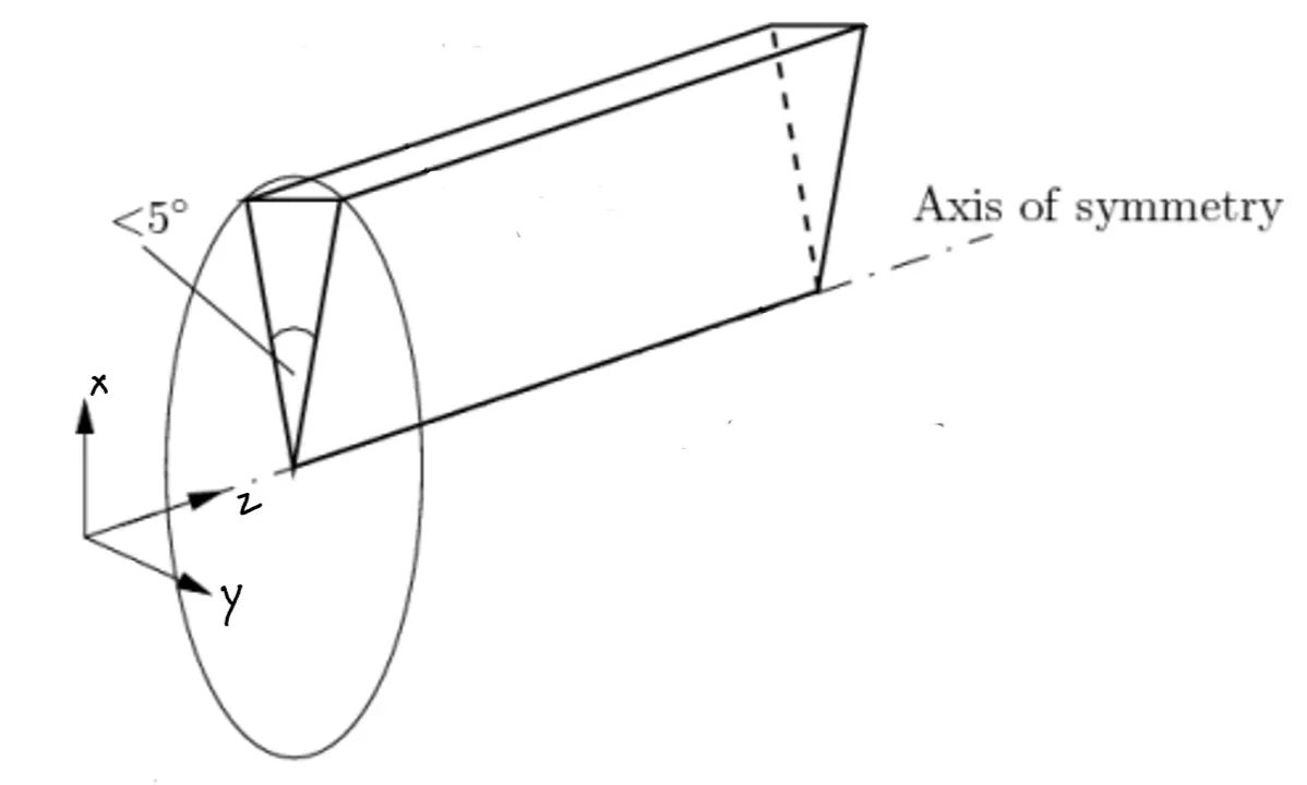
For the results, we need to observe the change in velocity profile and pressure drop across the length of the pipe. We also need to calculate the magnitude of shear stress acting on the walls of the domain. At last, we need to validate your obtained CFD results with the analytical solutions calculated from the Hagen–Poiseuille equations, to assure the fidelity of the numerical results. Assume constant velocity inlet and constant zero gauge pressure outlet as the initial boundary conditions. The flow velocity depends on the Reynold number, so in our case for the laminar region, consider the value of inlet flows Reynolds number `Re = 2100`. Run the simulation for enough time to observe all the essential changes with the suitable value of time step such that it satisfies our CFL condition. With appropriate Geometry, Mesh, Boundary and initial conditions are created by modifying the script files from the respective solver. All the physical properties and other essential parameters required to run the simulation are once again written below:

Wedge angle(`theta`) = `4^o`

Diameter of pipe (`D`) = `0.03m`

Outlet guage pressure (`P_o`) = `0 Pa`

Density of working fluid (water)(`rho`) = `997 kg//m^3`

Temperature of working fluid (`T`) = `20^0C`

Dynamic Viscosity (`mu`) = `0.997 ** 10^-3 Pa . sec`

`nu = mu/rho`

Kinematic viscosity (`nu`) = `1 ** 10^-6 m^2 // sec`

The length of the pipe should be choosed in such a way that it should be greater than the effective length in order to check the fedility of obtained results (`V_max` and `triangleP`) using Hagen Poiseuille law.

Hagen Poiseuille law:

In nonideal fluid dynamics, the Hagen–Poiseuille equation, also known as the Hagen–Poiseuille law, Poiseuille law or Poiseuille equation, is a physical law that gives the pressure drop in an incompressible and Newtonian fluid in laminar flow flowing through a long cylindrical pipe of constant cross section.

`=> "Volume Flow Rate"= Q = (DeltaPpiD^4)/(128muL)`

`thereforeDeltaP =( 128muQL_[fdr])/( piD^4)`

we know that `Q=VA=VpiR^2`, substituting this in above equation

`=> DeltaP=(32VmuL_[fdr])/(D^2)`

where `L_[fdr} =` Length of fully developed region

The assumptions of the equation are that the fluid is incompressible and Newtonian; the flow is laminar through a pipe of constant circular cross-section that is substantially longer than its diameter; and there is no acceleration of fluid in the pipe.

Hagen Poiseuille law is valid only in hydrodynamically fully developed region i.e.. only after the entrance region.

Entrance region:

In fluid dynamics, the entrance length is the distance a flow travels after entering a pipe before the flow becomes fully developed. Entrance length refers to the length of the entry region. When the boundary layer expands to fill the entire pipe, the developing flow becomes a fully developed flow, where flow characteristics no longer change with increased distance along the pipe. Many different entrance lengths exist to describe a variety of flow conditions. Hydrodynamic entrance length describes the formation of a velocity profile caused by viscous forces propagating from the pipe wall. Thermal entrance length describes the formation of a temperature profile. Awareness of entrance length may be necessary for the effective placement of instrumentation, such as fluid flow meters.

Hydrodanamic entrance length for a laminar flow is given by `=> L_[e,"laminar"] ~=0.05*Re*D`

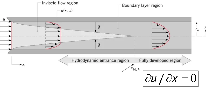
The region beyond the entrance region in which the velocity profile is fully developed and remains unchanged is called the hydrodynamically fully developed region. The flow is said to be fully developed when the normalized temperature profile and velocity profile remains unchanged across the length. The velocity still varies along the radial direction (the velocity gradient), but it remains constant in the axial direction.

The velocity profile in the fully developed region is parabolic in laminar flow and somewhat flatter (or fuller) in turbulent flow due to eddy motion and more vigorous mixing in the radial direction. The time-averaged velocity profile remains unchanged when the flow is fully developed. It can be shown mathematically as,

`=>(delU(r,x))/(delx) = 0=>U = U(r)`

Finding Analytical solution:

Average velocity or Inlet velocity: `=> Re=(rhoDV_[avg])/(mu)``=>2100=(997xx0.03xxV_[avg])/(0.997xx10^-3)``=>V_[avg] = 0.07m//s^`

Maximum velocity or Velocity at fully developed region: `=>V_max=2V_[avg](1-r^2/R^2)`

where, `r=R` at boundary

For fully developed flow, the maximum velocity will be at r=0.

Thus, `=> V_[max]=2*V_[avg]=>V_[max] = 2xx0.07=>0.14m//s`

Hydraulic entrance length: `=> L_[e,"laminar"] ~=0.05*Re*D=>L_[e,"laminar"] ~=0.05**2100**0.03m=>L_[e,"laminar"] ~=3.15m`

`therefore` we can see the fully developed region after the length of `L_e = 3.15m`. Let us consider the length of pipe as `L_T =5m`

`=>L_[fdr} = L_T - L_e => 5-3.15=>L_[fdr] = 1.85m`

The wall stress can be determined phenomenologically by the Darcy–Weisbach equation in the field of hydraulics, given a relationship for the friction factor in terms of the Reynolds number. In the case of laminar flow, for a circular cross section:

Darcy–Weisbach equation: `=>f=64/(Re)=>64/2100=>f=0.0305`

Pressure drop across the length in fully developed region: `=> DeltaP=(32V_[avg]muL_[fdr])/(D^2) =>(32**0.07**0.997**10^(-3)**1.85)/0.03^2=>DeltaP=4.594Pa`

Pressure drop can also be found using `=> DeltaP=f*L/D(rhoV_[avg]^2)/2`

Kinematic pressure drop in fully developed region: `=>DeltaP_k=(DeltaP)/rho=>4.594/997=>DeltaP_k=0.0046078`

Shear stress:

1. When the fluid is in motion, shear stresses are developed due to the particles in the fluid moving relative to one another.

2. For a fluid flowing in a pipe Fluid velocity will be zero at the pipe wall. Velocity will increase while moving towards the center of the pipe. Shear Force is normally present because the adjacent layer of the fluid move with different velocities compared to each other.

3. Fluids Obeying Newton's law where the values of “mu” are constant are known as Newtonian fluids. If ‘mu’ is constant, the shear stress is linearly dependent on the velocity gradient.

mathematically, Wall shear stress: `=>tau_w=f/4*(rhoV_[avg]^2)/2=>0.0305/4*(997xx0.07^2)/2=0.0186Pa`

Writing code in MATLAB and running the created code files in openFOAM:

Here comes the first part of this project. In this section, we are going to create the MATLAB script function that will generate the desired (blockMeshDict, controlDict, transportProperties, U, p, fvSolutions and fvSchemes) files which can then be used by OpenFOAM package to carry out further analysis.

The main objective of all this is to achieve automation in mesh generation and model set-up. This will ease the work by instantly generating the required script files for any given input parameters( like wedge angle or grading factor).

Matlab code:

Main code to take input of required data:

close all
clear all
clc

s = 1;                      %scaling factor
L = 5;                      %Length of pipe
r = 0.015;                  %Radius of pipe
theta = 2;                  %Angle of wedge wrt axis
rho = 997;                  %density of working fluid
Re =2100;                   %Renolds number
dx = 20;                    %Number of cells in X-direction
dy = 1;                     %Number of cells in y-direction
dz = 500;                   %Number of cells in z-direction
Xsg = 0.3;                   %Simple grading along X-direction
Ysg = 1;                     %Simple grading along Y-direction
Zsg = 1;                     %Simple grading along Z-direction
t = 210;                    %End time
dt = 0.001;                 %Time step
i =50;                      %writing interval
mu = 0.997*10^(-3);         %dynamic viscosity
FOAMscripts(s,L,r,theta,rho,Re,dx,dy,dz,Xsg,Ysg,Zsg,t,dt,i,mu)

Function code to create all required files:

function FOAMscripts(s,L,r,theta,rho,Re,dx,dy,dz,Xsg,Ysg,Zsg,t,dt,i,mu)
nue = mu/rho;               %kinematic viscosity
v = (Re*nue)/(2*r);         %Velocity
x1 = r*cosd(theta);         
y1 = r*sind(theta);
z1 = 0;
x2 = r*cosd(360-theta);
y2 = r*sind(360-theta);
z2 = L;
%common header lines

 line1='/*--------------------------------*-C++ -*--------------------------------*';
 line2='  =========                 |                                               ';
 line3='        /  F ield         |  OpenFOAM: The Open Source CFD Toolbox        ';
 line4='       /   O peration     |  Website: https://openfoam.org                ';
 line5='      /    A nd           |  Version: 8                                   ';
 line6='     /     M anipulation  |                                               ';
 line7='*-------------------------------------------------------------------------*/';
 line8='FoamFile';
 line9='// * * * * * * * * * * * * * * * * * * * * * * * * * * * * * * * * * * * * * //';

 mkdir 'Flow_through_a_pipe';
 mkdir 'Flow_through_a_pipe' 'system';
 mkdir 'Flow_through_a_pipe' 'constant';
 mkdir 'Flow_through_a_pipe' '0';
 %% blockmeshdict
 f=fopen('Flow_through_a_pipesystemblockMeshDict','w');
 fprintf(f,'%sn%sn%sn%sn%sn%sn%sn%sn{n%sn%sn%sn',line1,line2,line3,line4,line5,line6,line7,line8);
 fprintf(f,'tversion t2.0;ntformat tascii;ntclass ttdictionary;ntobject tblockMeshDict;n}n');
 %starting line
 fprintf(f,'%s',line9);
 %defining scaling factor
 fprintf(f,'nnconvertToMeters %d;nn',s);
 %defining vertices
 fprintf(f,'verticesn(nnt(0 0 0)nt(%f %f %f)nt(%f %f %f)nt(0 0 %f)nt(%f %f %f)nt(%f %f %f)n);n',x1,y1,z1,x1,y1,z2,z2,x2,y2,z1,x2,y2,z2);
 %defining blocks
 fprintf(f,'nblocksn(nthex (0 4 1 0 3 5 2 3) (%d %d %d) simpleGrading (%f %f %f)n);n',dx,dy,dz,Xsg,Ysg,Zsg);
 %defining edges
 fprintf(f,'nedgesn(ntarc 1 4 (%f %f %f)ntarc 2 5 (%f %f %f)n);n',x1/2,y1/2,z1,x2/2,y2/2,z2);
 %defining boundaries
 fprintf(f,'nboundaryn(nntaxisnt{ntttype empty;nttfacesntt(nttt(0 3 3 0)ntt);nt}n');
 fprintf(f,'tinletnt{ntttype patch;nttfacesntt(nttt(0 4 1 0)ntt);nt}n');
 fprintf(f,'toutletnt{ntttype patch;nttfacesntt(nttt(3 5 2 3)ntt);nt}n');
 fprintf(f,'tleftwallnt{ntttype wedge;nttfacesntt(nttt(4 0 3 5)ntt);nt}n');
 fprintf(f,'trightwallnt{ntttype wedge;nttfacesntt(nttt(0 1 2 3)ntt);nt}n');
 fprintf(f,'touterwallnt{ntttype wall;nttfacesntt(nttt(1 4 5 2)ntt);nt}nnn);n');
 %defining patch pairs
 fprintf(f,'nmergePatchPairsn(n);n');
 %ending line
 fprintf(f,'n%s',line9);
 fclose(f);
 %% control dict 
 f=fopen('Flow_through_a_pipesystemcontrolDict','w');
 fprintf(f,'%sn%sn%sn%sn%sn%sn%sn%sn{n%sn%sn%sn',line1,line2,line3,line4,line5,line6,line7,line8);
 fprintf(f,'tversion t2.0;ntformat ttascii;ntclass ttdictionary;ntlocationt"system";ntobject ttcontrolDict;n}n');
 %starting line
 fprintf(f,'%sn',line9);
 fprintf(f,'napplicationticoFoam;nnstartFromtstartTime;nnstartTimet0;nnstopAtttendTime;nnendTimett%f;nndeltaTtt%fs;',t,dt);
 fprintf(f,'nnwriteControlttimeStep;nnwriteIntervalt%d;nnpurgeWritet0;nnwriteFormattascii;nnwritePrecisiont6;nnwriteCompressiontoff;nntimeFormattgeneral;nntimePrecisiont6;nnrunTimeModifiablettrue;',i);
 %ending line
 fprintf(f,'nn%s',line9);
 fclose(f);
 %% fvSchemes
 f=fopen('Flow_through_a_pipesystemfvSchemes','w');
 fprintf(f,'%sn%sn%sn%sn%sn%sn%sn%sn{n%sn%sn%sn',line1,line2,line3,line4,line5,line6,line7,line8);
 fprintf(f,'tversion t2.0;ntformat ttascii;ntclass ttdictionary;ntlocationt"system";ntobject ttfvSchemes;n}n');
 %starting line
 fprintf(f,'%sn',line9);
 fprintf(f,'nddtSchemesn{ntdefaultttEuler;n}nngradSchemesn{ntdefaultttGauss linear;ntgrad(p)ttGauss linear;n}nndivSchemesn{ntdefaultttnone;ntdiv(phi,U)tGauss linear;n}nn');
 fprintf(f,'laplacianSchemesn{ntdefaultttGauss linear orthogonal;n}nninterpolationSchemesn{ntdefaultttlinear;n}nnsnGradSchemesn{ntdefaultttorthogonal;n}');
 %ending line
 fprintf(f,'nn%s',line9);
 fclose(f);
 %% fvSolution
 f=fopen('Flow_through_a_pipesystemfvSolution','w');
 fprintf(f,'%sn%sn%sn%sn%sn%sn%sn%sn{n%sn%sn%sn',line1,line2,line3,line4,line5,line6,line7,line8);
 fprintf(f,'tversion t2.0;ntformat ttascii;ntclass ttdictionary;ntlocationt"system";ntobject ttfvSolution;n}n');
 %starting line
 fprintf(f,'%sn',line9);
 fprintf(f,'nsolversn{ntpnt{nttsolverttPCG;nttpreconditionertDIC;ntttolerancet1e-06;nttrelToltt0.05;nt}n');
 fprintf(f,'ntpFinalnt{ntt$p;nttrelToltt0;nt}nntUnt{nttsolverttsmoothSolver;nttsmoothertsymGaussSeidel;ntttolerancet1e-05;nttrelToltt0;nt}n}n');
 fprintf(f,'nPISOn{ntnCorrectorst2;ntnNonOrthogonalCorrectorst0;ntpRefCellt0;ntpRefValuet0;n}');
 %ending line
 fprintf(f,'nn%s',line9);
 fclose(f);
 %% transport properties
 f=fopen('Flow_through_a_pipeconstanttransportProperties','w');
 fprintf(f,'%sn%sn%sn%sn%sn%sn%sn%sn{n%sn%sn%sn',line1,line2,line3,line4,line5,line6,line7,line8);
 fprintf(f,'tversion t2.0;ntformat ttascii;ntclass ttdictionary;ntlocationt"constant";ntobject tttransportProperties;n}n');
 %starting line
 fprintf(f,'%sn',line9);
 %defining kinematic viscosity of water
 fprintf(f,'nnutt[0 2 -1 0 0 0 0]  %f;n',nue);
 %ending line
 fprintf(f,'n%s',line9);
 fclose(f);
 %% pressure
 f=fopen('Flow_through_a_pipep','w');
 fprintf(f,'%sn%sn%sn%sn%sn%sn%sn%sn{n%sn%sn%sn',line1,line2,line3,line4,line5,line6,line7,line8);
 fprintf(f,'tversion t2.0;ntformat ttascii;ntclass ttvolScalarField;ntobject ttP;n}n');
 %starting line
 fprintf(f,'%sn',line9);
 %defining pressure conditions
 fprintf(f,'ndimensionst[0 2 -2 0 0 0 0];nninternalFieldtuniform 0;nnboundaryFieldn{n');
 fprintf(f,'tinletnt{ntttypetzeroGradient;nt}ntoutletnt{ntttypetfixedValue;nttvaluetuniform 0;nt}');
 fprintf(f,'ntaxisnt{ntttypetempty;nt}ntleftwallnt{ntttypetwedge;nt}ntrightwallnt{ntttypetwedge;nt}ntouterwallnt{ntttypetzeroGradient;nt}nn}');
 %ending line
 fprintf(f,'n%s',line9);
 fclose(f);
 %% velocity
 f=fopen('Flow_through_a_pipeU','w');
 fprintf(f,'%sn%sn%sn%sn%sn%sn%sn%sn{n%sn%sn%sn',line1,line2,line3,line4,line5,line6,line7,line8);
 fprintf(f,'tversion t2.0;ntformat ttascii;ntclass ttvolVectorField;ntobject ttU;n}n');
 %starting line
 fprintf(f,'%sn',line9);
 %defining velocity conditions
 fprintf(f,'ndimensionst[0 1 -1 0 0 0 0];nninternalFieldtuniform (0 0 0);nnboundaryFieldn{n');
 fprintf(f,'toutletnt{ntttypetzeroGradient;nt}ntinletnt{ntttypetfixedValue;nttvaluetuniform (0 0 %f);nt}',v);
 fprintf(f,'ntaxisnt{ntttypetempty;nt}ntleftwallnt{ntttypetwedge;nt}ntrightwallnt{ntttypetwedge;nt}ntouterwallnt{ntttypetnoSlip;nt}nn}');
 %ending line
 fprintf(f,'n%s',line9);
 fclose(f);

1. Creating geometry, automeshing and simple grading:

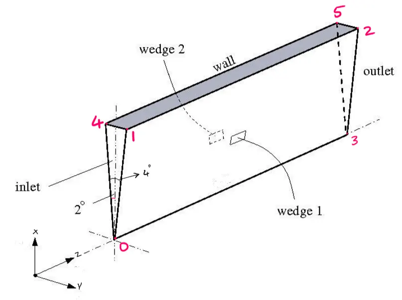
The boundary conditions and the order of vertices are shown below

blockMeshDict file:

/*--------------------------------*-C++ -*--------------------------------*
  =========                 |                                               
        /  F ield         |  OpenFOAM: The Open Source CFD Toolbox        
       /   O peration     |  Website: https://openfoam.org                
      /    A nd           |  Version: 8                                   
     /     M anipulation  |                                               
*-------------------------------------------------------------------------*/
FoamFile
{
	version 	2.0;
	format 	ascii;
	class 		dictionary;
	object 	blockMeshDict;
}
// * * * * * * * * * * * * * * * * * * * * * * * * * * * * * * * * * * * * * //

convertToMeters 1;

vertices
(

	(0 0 0)
	(0.014991 0.000523 0.000000)
	(0.014991 0.000523 5.000000)
	(0 0 5.000000)
	(0.014991 -0.000523 0.000000)
	(0.014991 -0.000523 5.000000)
);

blocks
(
	hex (0 4 1 0 3 5 2 3) (20 1 500) simpleGrading (0.300000 1.000000 1.000000)
);

edges
(
	arc 1 4 (0.007495 0.000262 0.000000)
	arc 2 5 (0.007495 -0.000262 5.000000)
);

boundary
(

	axis
	{
		type empty;
		faces
		(
			(0 3 3 0)
		);
	}
	inlet
	{
		type patch;
		faces
		(
			(0 4 1 0)
		);
	}
	outlet
	{
		type patch;
		faces
		(
			(3 5 2 3)
		);
	}
	leftwall
	{
		type wedge;
		faces
		(
			(4 0 3 5)
		);
	}
	rightwall
	{
		type wedge;
		faces
		(
			(0 1 2 3)
		);
	}
	outerwall
	{
		type wall;
		faces
		(
			(1 4 5 2)
		);
	}


);

mergePatchPairs
(
);

// * * * * * * * * * * * * * * * * * * * * * * * * * * * * * * * * * * * * * //

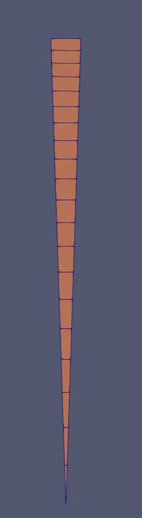
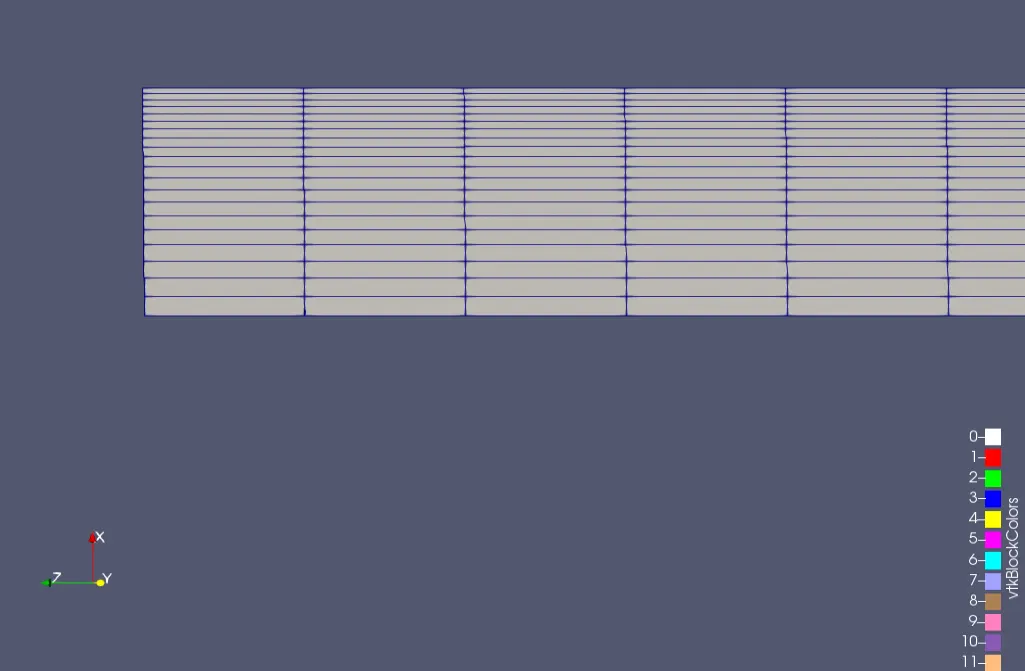
The mesh is generated using file named blockMeshDict located in system directory. blockMesh reads this dictionary, generates the mesh, and writes out the mesh data to points and faces, cells, and boundary files in the constant/polyMesh directory of a case.

The computational domain is discretized using 20cells, 1cell and 500cells with simple grading of 0.3,1,1 in X,Y,Z directions respectively.

We can check the meshing by entering paraFoam in terminal

2. Setting transport properties:

In OpenFOAM, the physical parameters for a specific flow problem are described in the file called TransportProperties. This file is located in the constant directory under our case file. In our case, we have assumed that our fluid is a Newtonian fluid, and the kinematic viscosity of fluid flow is given as `1e-6`.

/*--------------------------------*-C++ -*--------------------------------*
  =========                 |                                               
        /  F ield         |  OpenFOAM: The Open Source CFD Toolbox        
       /   O peration     |  Website: https://openfoam.org                
      /    A nd           |  Version: 8                                   
     /     M anipulation  |                                               
*-------------------------------------------------------------------------*/
FoamFile
{
	version 	2.0;
	format 		ascii;
	class 		dictionary;
	location	"constant";
	object 		transportProperties;
}
// * * * * * * * * * * * * * * * * * * * * * * * * * * * * * * * * * * * * * //

nu		[0 2 -1 0 0 0 0]  0.000001;

// * * * * * * * * * * * * * * * * * * * * * * * * * * * * * * * * * * * * * //

3. Specifing End time and time step:

While selecting numerical schemes to solve the discretized governing equations, the only accuracy is not enough. Our numerical scheme should be both stable and accurate. We say a numerical scheme is stable when truncation error does not increase in amplitude after each time step. So, there exist stability criteria that calculate the extreme values of the time step and space step for such numerical schemes to attain stability. For our problem statement, we use CFL ( Courant–Friedrichs–Lewy condition ) stability criteria to get our stability condition.

In OpenFOAM, input data relating to the control of time and reading and writing of the solution data are read in from the controlDict file. For the end time, we wish to reach the steady-state solution where the flow is stable and constant. As a general rule, the fluid should pass through the domain three times to reach a steady-state in laminar flow. So, after calculation, we discover that 210s is sufficient, so we shall adopt this value. To specify this end time, we must specify the stopAt keyword as endTime and then set the endTime keyword to 210s. Now we need to set the time step, represented by the keyword deltaT. To achieve temporal accuracy and numerical stability when running icoFoam, a Courant number of less than 1 is required. The Courant number is defined for one cell as:

`C = |V|*(delta t)/(delta x)`

where, `deltat =`time step; `V =`velocity; `deltax =`cell size.

The flow velocity varies across the domain, and we must ensure that `C <1` for every cell. After all the calculations, we conclude that, to achieve a Courant number less than or equal to 1 throughout the domain, the time step should be set to `deltat <= 0.001`

/*--------------------------------*-C++ -*--------------------------------*
  =========                 |                                               
        /  F ield         |  OpenFOAM: The Open Source CFD Toolbox        
       /   O peration     |  Website: https://openfoam.org                
      /    A nd           |  Version: 8                                   
     /     M anipulation  |                                               
*-------------------------------------------------------------------------*/
FoamFile
{
	version 	2.0;
	format 		ascii;
	class 		dictionary;
	location	"system";
	object 		controlDict;
}
// * * * * * * * * * * * * * * * * * * * * * * * * * * * * * * * * * * * * * //

application	icoFoam;

startFrom	startTime;

startTime	0;

stopAt		endTime;

endTime		210.000000;

deltaT		0.001000s;

writeControl	timeStep;

writeInterval	50;

purgeWrite	0;

writeFormat	ascii;

writePrecision	6;

writeCompression	off;

timeFormat	general;

timePrecision	6;

runTimeModifiable	true;

// * * * * * * * * * * * * * * * * * * * * * * * * * * * * * * * * * * * * * //

4. Setting initial and boundary conditions (U & p):

Governing equations are the same for every CFD problem, and then there should be something that makes our results unique for every flow problem. This is done by setting up Initial and Boundary conditions of velocity (U) and Pressure(p) which are stored in 0 directory.

Velocity script

/*--------------------------------*-C++ -*--------------------------------*
  =========                 |                                               
        /  F ield         |  OpenFOAM: The Open Source CFD Toolbox        
       /   O peration     |  Website: https://openfoam.org                
      /    A nd           |  Version: 8                                   
     /     M anipulation  |                                               
*-------------------------------------------------------------------------*/
FoamFile
{
	version 	2.0;
	format 		ascii;
	class 		volVectorField;
	object 		U;
}
// * * * * * * * * * * * * * * * * * * * * * * * * * * * * * * * * * * * * * //

dimensions	[0 1 -1 0 0 0 0];

internalField	uniform (0 0 0);

boundaryField
{
	outlet
	{
		type	zeroGradient;
	}
	inlet
	{
		type	fixedValue;
		value	uniform (0 0 0.070000);
	}
	axis
	{
		type	empty;
	}
	leftwall
	{
		type	wedge;
	}
	rightwall
	{
		type	wedge;
	}
	outerwall
	{
		type	noSlip;
	}

}
// * * * * * * * * * * * * * * * * * * * * * * * * * * * * * * * * * * * * * //

Pressure script

/*--------------------------------*-C++ -*--------------------------------*
  =========                 |                                               
        /  F ield         |  OpenFOAM: The Open Source CFD Toolbox        
       /   O peration     |  Website: https://openfoam.org                
      /    A nd           |  Version: 8                                   
     /     M anipulation  |                                               
*-------------------------------------------------------------------------*/
FoamFile
{
	version 	2.0;
	format 		ascii;
	class 		volScalarField;
	object 		P;
}
// * * * * * * * * * * * * * * * * * * * * * * * * * * * * * * * * * * * * * //

dimensions	[0 2 -2 0 0 0 0];

internalField	uniform 0;

boundaryField
{
	inlet
	{
		type	zeroGradient;
	}
	outlet
	{
		type	fixedValue;
		value	uniform 0;
	}
	axis
	{
		type	empty;
	}
	leftwall
	{
		type	wedge;
	}
	rightwall
	{
		type	wedge;
	}
	outerwall
	{
		type	zeroGradient;
	}

}
// * * * * * * * * * * * * * * * * * * * * * * * * * * * * * * * * * * * * * //

5. Post processing and results:

Here, the simulation is ran by using icoFoam Solver using PISO algorithm.

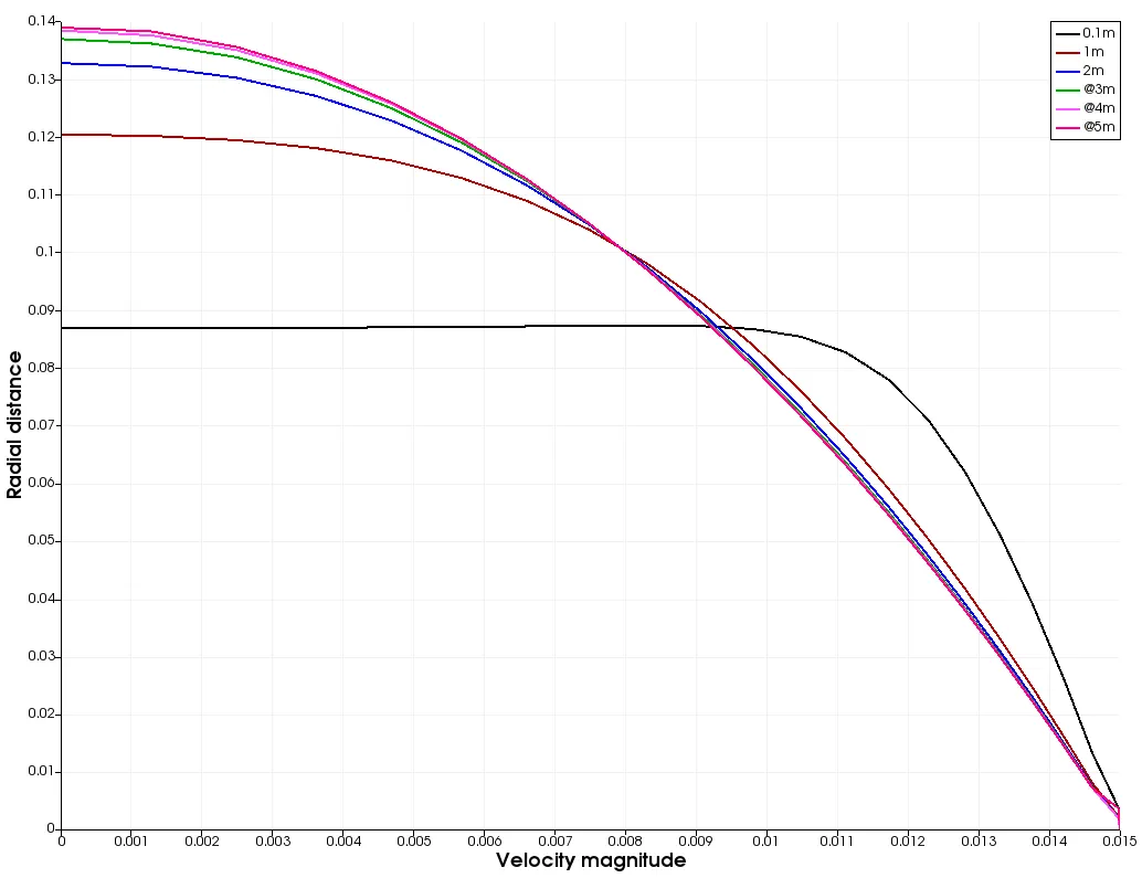
As the entrance length obtained from the formula is 3.15m, all the calucaltions are made between the length 3.15 and 5m

Plot1 - Velocity magnitude at different axial distances of pipe

Plot2 - Velocity magnitude along axial distance of pipe

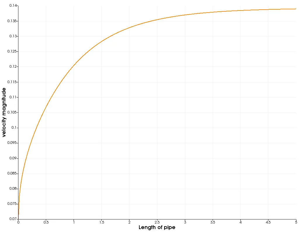
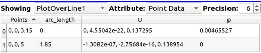
The above data is at the points `3.15m` and `5m` of pipe.

Length of fully developed region(arc length) is `L_[fdr]=1.85m`

Max velocity is `V_(max)=0.138954m//s`

Pressure drop `DeltaP= 0.004655Pa`

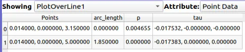
Wall shear stress is `tau_w=0.0175`

wall shear stress after entrance length is almost equivalent till the end of the pipe `approx0.017`

Conclusion

The simulation results were in accordance with the Values obtained from the Hagen Poiseuille Equations with These errors obtained may be reduced further by finer grids, but the computation time would increase. This is the reason many different grids were not simulated. The selection of the length of the pipe can be made by identifying the development of the velocity profile also the material selection for the pipe is made by considering the wall shear stress value.

With this, we can conclude that the reduced wedge model was an adequate substitute for the complete circular pipe. Besides the fact that it reduced the computational efforts extensively, the results obtained through this were also quite accurate.