Build simulink models of force applied on cutting tool, implement equation of z=3x2-5y+18 and understanding the Mass-spring-damper system

Aim :-

Build simulink models of force applied on cutting tool, implement equation of z=3x²-5y+18 and understanding the Mass-spring-damper system.

Objective :-

1. The force on a cutting tool of a shaping machine varies over the length of cut as follows:

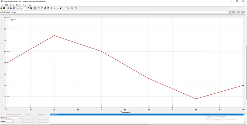
Distance (mm) 0 20 40 60 80 100

Force (kN) 60 72 65 53 44 50

Determine the work done as the tool moves through a distance of 100 mm.

2. Create two array data sets x = [22 3 55.6 9 12 10] and y = [5 31 95 56.3 77 61] from the command window. Create a Simulink model to implement equation z=3x²-5y+18 Store result values using To File block.

3. Go to Matlab Help. Type the keyword ‘Mass-Spring-Damper in Simulink and Simscape’. Open the model and solve the following problems:

• Derive the governing equation for the model
• Change the value of mass, damper, and spring for the Simscape model and plot the result. Change the value of Mass ,displacement as x0=2 in the Simulink model and plot the results.
• Make the response from Simscape and Simulink as two separate displays.

ANSWER :-

1] Part 1 :-

The force on a cutting tool of a shaping machine varies over the length of cut as follows:

Distance (mm) 0 20 40 60 80 100

Force (kN) 60 72 65 53 44 50

Determine the work done as the tool moves through a distance of 100 mm.

Basic Blocks used in Simulink Model :-

1. Signal Builder Block :- The Signal Builder block allows you to create interchangeable groups of piecewise linear signal sources and use them in a model.
2. Integrator Block :- The Integrator block outputs the value of the integral of its input signal with respect to time.
3. Display Block :- The Display block shows the value of the input data.
4. Scope :- Display signals generated during simulation.

Simulink Model :-

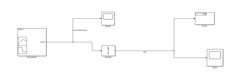
Google Drive Link :- https://drive.google.com/file/d/1LC1VaWW_XZRMcR5o-0RF_VRNr3Sgvbu3/view?usp=sharing

Explanation :-

1. Initially, we have used Signal builder block so that we can put force and displacement values as input signal values. The same is as under;

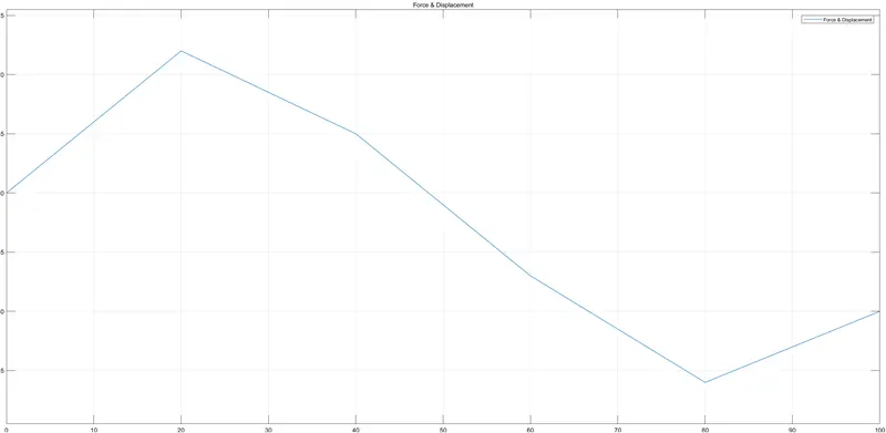
2. Thereafter, we have connected scope block to output terminal of signal builder block to see input signals of Force v/s Displacement graph.

The same is as under;

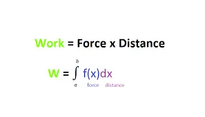
3. As we aware that, we have to find the work done by cutting tool through a total distance of 100 mm. Hence, we know that we have to use following equation to get the desired result.

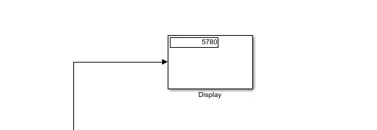
4. Hence, we have used integrator block to integrate all input values. Thereafter, we have connected display block to integrator block to check the total work done by cutting tool through a distance of 100 mm.

The displayed value of work done is as under;

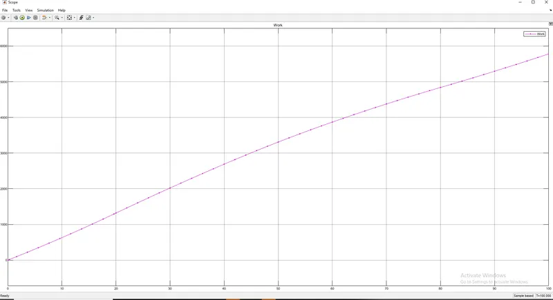
5. Also, we have connected scope block to output terminal of integrator block to see the graph of work done by cutting tool.

Output Graph :-

Conclusion :-

• We have connected Signal Builder with Integrator to make Integral of distance with respect to time which is nothing but displacement.
• It gives a total area between the path and the boundary.In this case the path is from 0-100(Time) and From (Point 1 - Point 6) is the distance of the boundary from the path. Finally, Net Workdone has been calculated.
• While going through the graph, we observed that when force applied is directly proportional to the work done on the cutting tool.

PART 2:- Create two array data sets x = [22 3 55.6 9 12 10] and y = [5 31 95 56.3 77 61] from the command window. Create a Simulink model to implement equation z=3x²-5y+18 Store result values using To File block.

Blocks used in the simulink model :-

1. Square Block :- This block performs square operation.
2. Product Block :- This block performs multiplication of input values and gives output values.
3. Sum Block :- This block is used to perform addition and substraction based on user input.
4. Display Block :- This block is used to display output values
5. To file Block :- This block incrementally writes data into a variable in the specified MAT-file.
6. Constant Block :- Output the constant specified by the 'Constant value' parameter.

Simulink Model :-

Google Drive Link :-

https://drive.google.com/file/d/18f9tpVS4-ccuof_H23B4rDUGGiv9_nt0/view?usp=sharing

Explanation :-

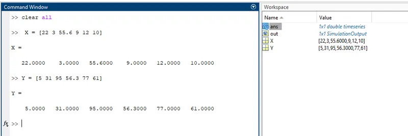
1. Initially, we have created two input arrays X = [22 3 55.6 9 12 10] and Y = [5 31 95 56.3 77 61] in the command window and the same is as under;

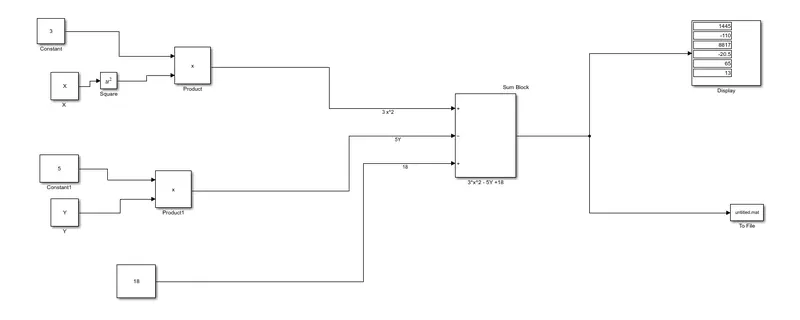
2. Thereafter, we have attached constant blocks of value '3' and 'X' value block and further, connected to product block to get output value of 3x^2.

3. Similarly, we have attached constant blocks for value '5' and 'Y' value block and further, connected to product block to get output value of 5Y.

4. Then, we have connected input signal of 3x^2, 5Y and 18 to the sum block, so that output has been achieved for equation z= 3x^2 -5Y +18.

5. At the output of sum block, we have attached display block to see output values for particular given equation.

For particular equation, we got the output values as under;

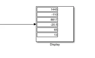
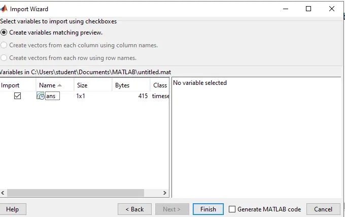
6. Also, we have connected To file block to the output port of sum block so that all generated output values can be stored in 'untitled.mat' matlab file. The same is as under;

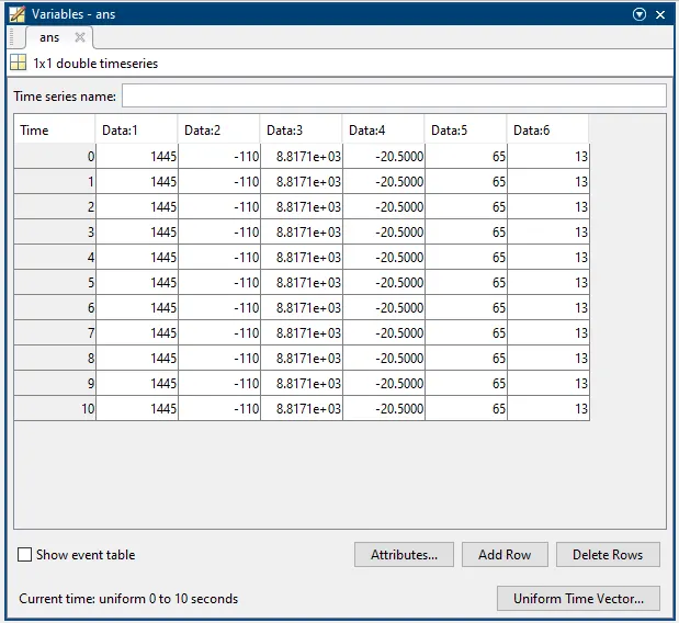
7. After opening, we have created the variable named 'ans' and the same was shown in the workspace. Here, we have run the simulation for 10 sec,hence total 6 values were generated for every seconds starting from 0 to 10 sec.

PART 3 :- Go to Matlab Help. Type the keyword ‘Mass-Spring-Damper in Simulink and Simscape’. Open the model and solve the following problems:

1. Derive the governing equation for the model
2. Change the value of mass, damper, and spring for the Simscape model and plot the result. Change the value of Mass ,displacement as x0=2 in the Simulink model and plot the results.
3. Make the response from Simscape and Simulink as two separate displays.

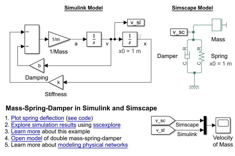
Theory :-

• The mass of the dynamic system is lumped into a single point mass in the MSD system. The inertial effect of the dynamic system is related through this lumped mass.
• The stored energy/internal energy of the dynamic system is modelled as a one-dimensional spring in the MSD system.
• The spring is able to store energy inside when it is stretched or compressed from its original length.
• The energy dissipated out of the dynamic system is modelled through a one-dimensional damper in the MSD system.
• The viscous damper, for instance, is able to dissipate energy as heat outside the dynamic system.

F.B.D. of Spring-Mass-Damper system :-

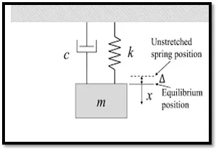
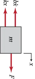
Governing Equation of the model :-

While going through the F.B.D. of Spring-Mass damper system, we observed that block of mass (m) is having displacement of x meter due to the force (F). However, damper and spring were having their damping force and spring force respectively as resisting forces to external force (F).

Therefore,

Spring force (Fs) = kx;

Coulomb Damping Force (Fd) = bx';

where,

k= Spring constant (N/m)

b= Damping coefficient (N/(m/s))

x= Displacement (m)

x' = Velocity (m/s) = dx/dt

m = block of mass (Kg)

Considering all the forces the Y direction, we get

F = -bx' - kx ......... (1)(Downward forces considered positive and Upward forces considered negative)

also,

we know that force (F) =Mass x Acceleration

However,

Acceleration = (d^2)x/dt^2 = x'' (m/s^2)

Hence, putting the values of force (F) in the equation(1), we get,

F = -bx' - kx

Mass x Acceleration = -bx' - kx

m [(d^2)x/dt^2] = -bx' - kx ...............(2)

Dividing the equation (2) by mass(m), we get

[(d^2)x/dt^2] = (-b/m)x' - (k/m)x

Resubstituting the value of acceleration =(d^2)x/dt^2 = x'' in the above equation, we get,

x" = (-b/m)x' - (k/m)x

Rearranging the equation, we get,

x"+(b/m)x' +(k/m)x = 0 .............(3)

The above equation (3) represents governing equation of above Spring-mass-damper system.

This equation is also called as Second order linear differential equation.

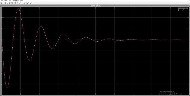
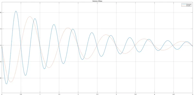
For default values of mass (m), damping (b) and spring constant(k), we have the output graph of velocity for simulink and simscape is as under;

mass (m) = 3.6 kg

Damping coefficient (b) = 10 N/(m/s)

Spring constant (k) = 400 N/m

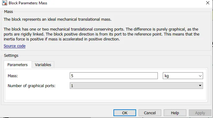
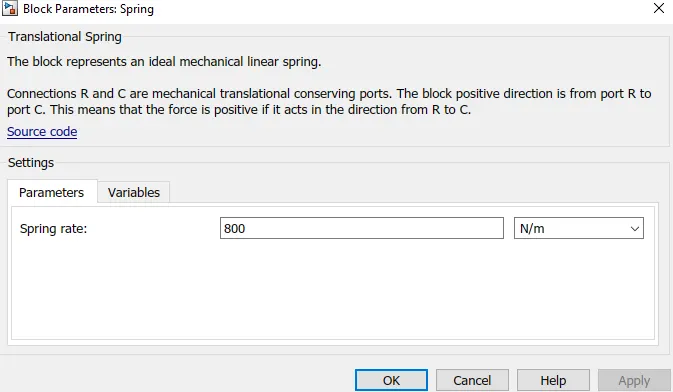
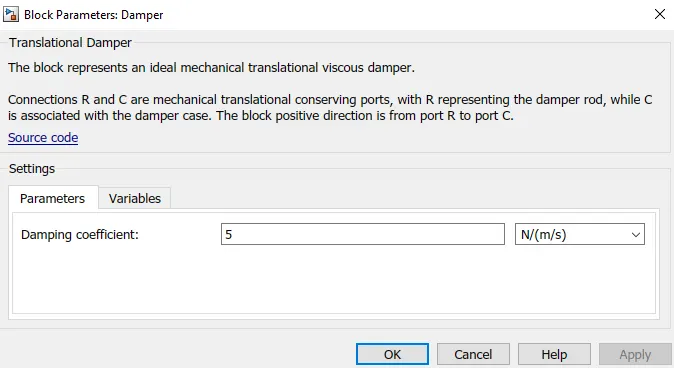
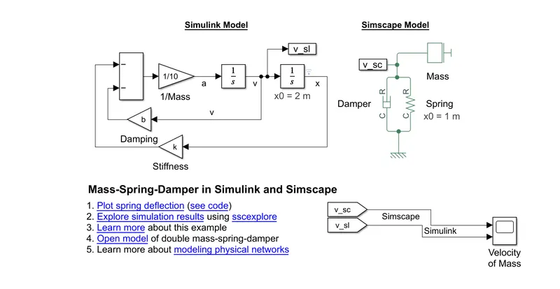
When we change the input value of mass, damper and spring for simscape model and changing the value of mass, displacement as x0=2, we get

For simulink model at x0=2m,

m=10 kg

b= 10 N/(m/s)

k= 400 N/m

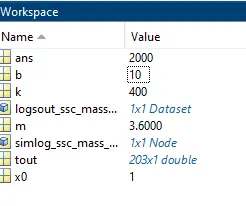
For simscape model at x0=1m,

m =5 kg

b= 5 N/(m/s)

k=800 N/m

Output Graph :-

Observations:-

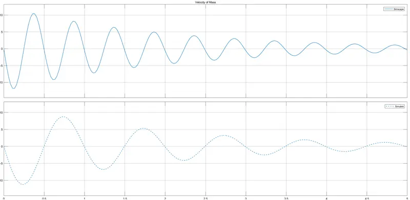
• Here, we have decreased the damping coefficient value(b) in simscape model, hence observed that amplitude and oscillation of signal for simcape model got increased. Also, we have increased the value for spring constant(k), result of increase of amplitude and oscillation for simscape model was observed as compared to simulink model.

For creating two seperate displays/ graphs, we have to modify the model as under;

Google Drive Model link :-

https://drive.google.com/file/d/19xA2PhqwfA0Syyt4PIwqpl5G57liXQCr/view?usp=sharing

Output Graphs:-

Conclusion :-

1. While going through the graph, we observed that when we decrease the damping coefficient value(b), amplitude and oscillation of the signal increases.
2. Also, we noted that when we increase the spring constant (k) value, oscillation of the signal got increased.
3. Hence, we can conclude that spring constant(k) is directly proportional to oscillation of the signal and damping coefficient value(b) is inversely proportional to the oscillation.