NUMERICAL STUDY OF AERODYNAMICS OF AN AHMED BODY

AIM:

• Performing the grid independency test and provide the values of drag and lift with each case.
• Running the simulation for the velocity of 25 m/sec with the default air properties in fluent.
• Ahmed's body and its importance.

OBJECTIVES:

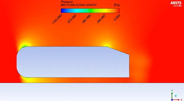
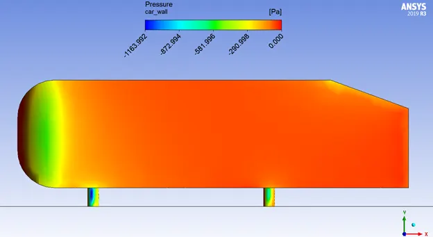
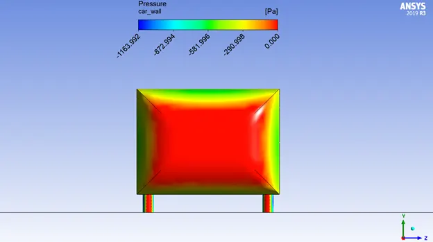
1. The reason for the negative pressure in the wake region.
2. The significance of the point of separation.
3. Velocity and pressure contours.
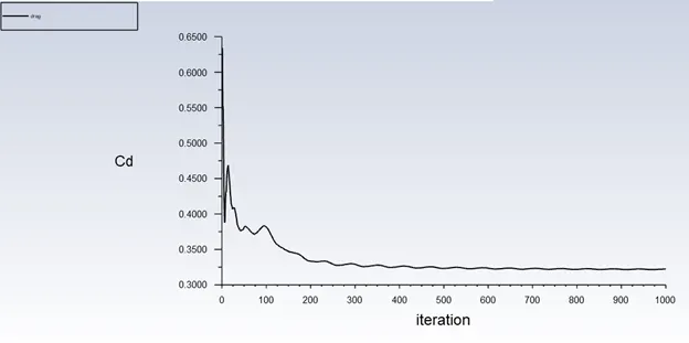
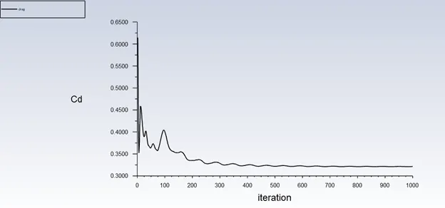
4. The drag coefficient plot for a refined mesh case.
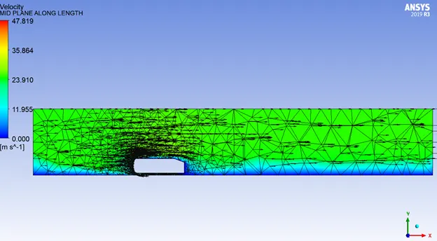
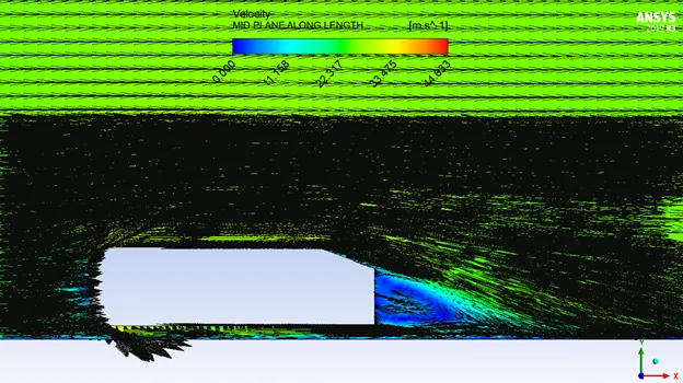
5. The vector plot clearly showing the wake region.
6. For velocity of 25m/sec, the drag coefficient should be around 0.33.

AHMED BODY:

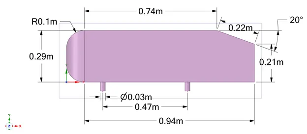
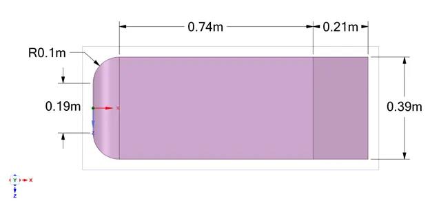
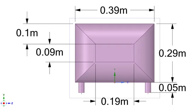
The Ahmed body is a generic car body (a simplified vehicle model). The airflow around the Ahmed body captures the essential flow features around an automobile and was first defined and characterized in the experimental work of Ahmed. Although it has a very simple shape, Ahmed body allows us to capture characteristic features that are relevant to bodies in the automobile industry.

This model is also used to describe the turbulent flow field around a car-like geometry. Once the numerical model in validated, it is used to design new models of the car.

People working in vehicle aerodynamics use Ahmed body to validate their numerical model because the experimental data from wind tunnel testing is available for Ahmed body. Once the numerical model in validated, it is used to design new models of the car.

AHMED BODY MODEL:

SIIDE VIEW:

TOP VIEW:

FRONT VIEW:

FLOW DOMAIN:

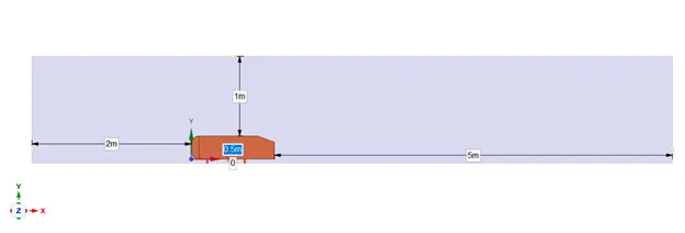
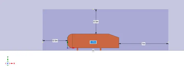
Using enclosure option in ANSYS SpaceClaim to create a flow domain.

SIDE VIEW:

REAR VIEW:

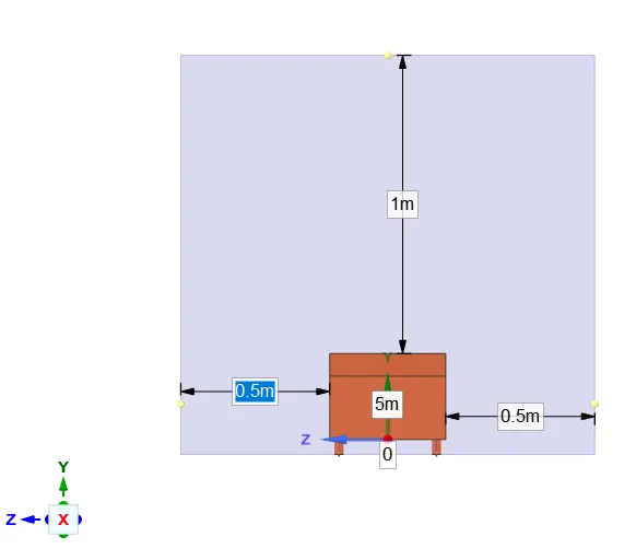
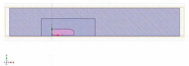
For more accurate simulation of the wake region another enclosure (to add a finer mesh) is added to the Ahmed body.

Used the interference tool and Share Topology = Share

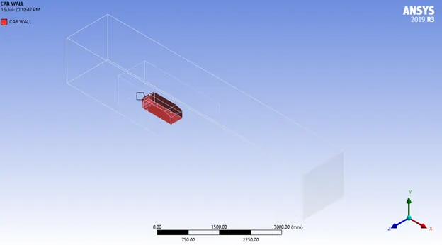
BOUNDARIES:

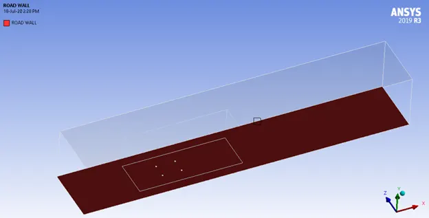
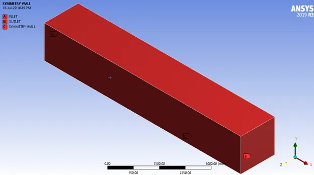
STEADY-STATE SIMULATION

Material used: Air (properties below)

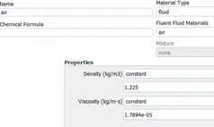
ρ = 1.225 kg/m³

μ = 1.7894 × 10^-5 kg/m-s

L = Length of Ahmed Body = 1.04 m

Re_L = `(ρ*V*L)/μ`

V = 25 m/s

Re_L = `(1.225×25× 1.04)/(1.7894 × 10^-5 )` = 1779926.23

Hence, Turbulence Model. Since the wall functions needs to be considered to get wall precise values, k-epslon model is used in the simulation.

Solution Method: SIMPLE

Mach Number, M = `(velocity of fluid)/(velocity of sound)`

Velocity of fluid = V = 25 m/s

Velocity of Sound = `sqrt ((γ×P)/ρ)`

𝛄 = 1.4

P = 101325 Pa

Velocity of Sound = `sqrt((1.4×101325)/1.225)` = 340.2939 m/s

M = `25/340.2939` = 0.0734

M < 0.3 (Incompressible Flow)

Hence, Pressure based solver is used.

BOUNDARY CONDITIONS:

INLET: Velocity Magnitude = 25 m/s

OUTLET: Pressure (Gauge) = 0 Pa

SYMMETRY WALL - Type: Symmetry

ROAD WALL - Type: Wall, no slip condition

CAR WALL - Type: Wall, no slip condition

BASELINE MESH:

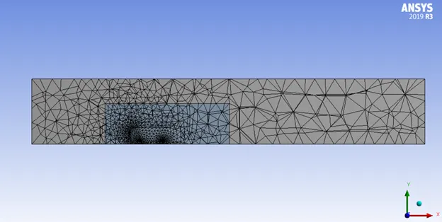
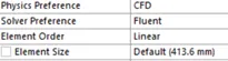
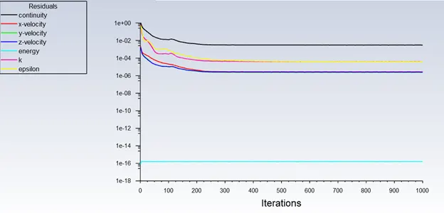
Number of iterations given to run = 1000

Number of iterations to converge = 300

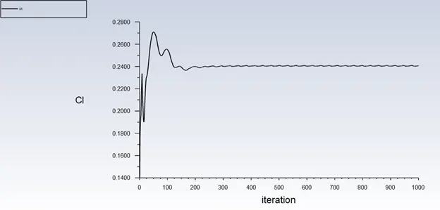
Projected Area = 0.13148199 m²

Length =1.04 m

Lift coefficient = 0.24052832

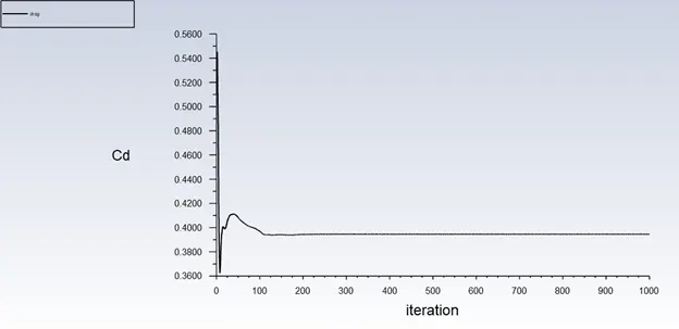
Drag Coefficient = 0.39467476

Velocity & Pressure Contour:

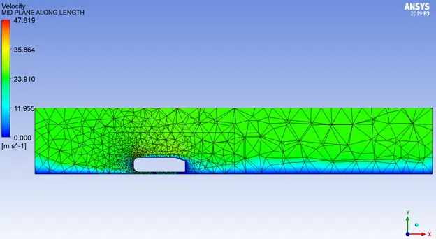
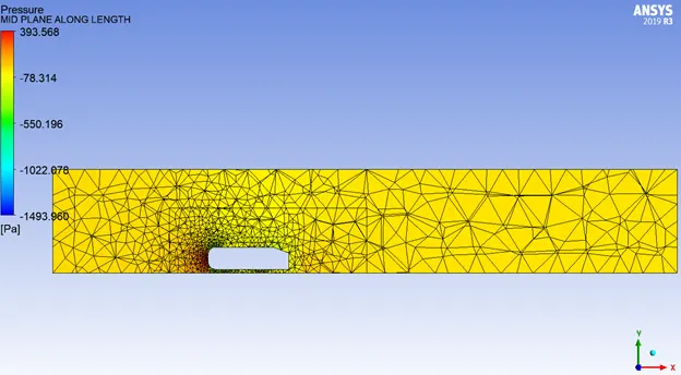
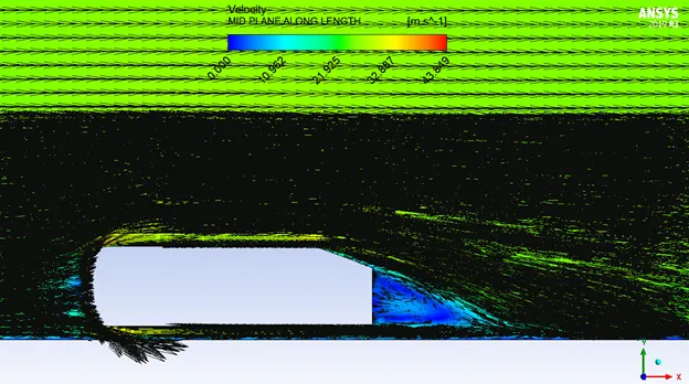
Velocity Vector Plot:

REFINED MESH 1

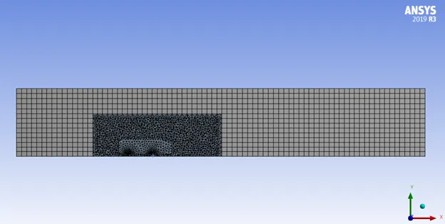
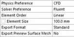
Used Mesh Method Multizone to add Hexahedral Mesh to the outer enclosure and the element size was set to 100 mm. Another body sizing was added to the inner enclosure with element size 50 mm.

Add inflation layer:

Wall spacing = 5 mm

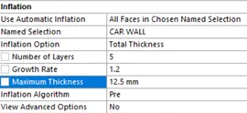
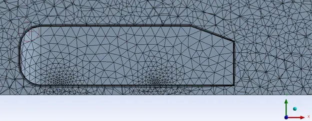
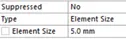
Face Sizing on the cylindrical support of the Ahmed body:

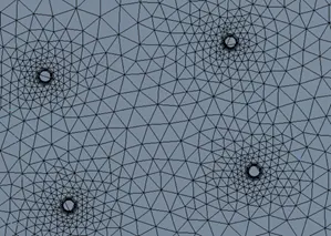
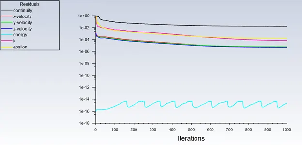
Number of iterations given to run = 1000

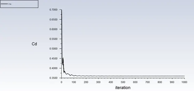
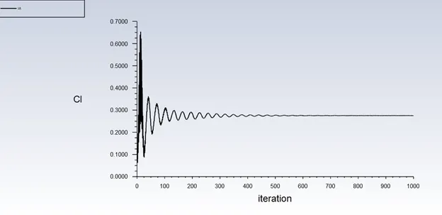
Number of iterations to converge = 310

Drag Coefficient = 0.35988549

Lift Coefficient = 0.27571222

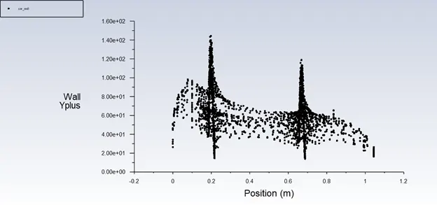
Y⁺ in range for k-epsilon model.

Velocity & Pressure Contour:

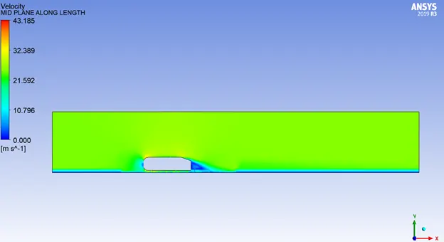
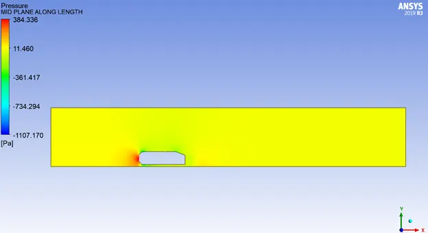
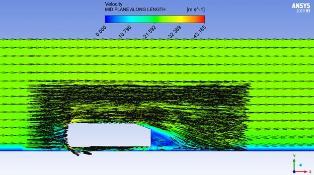
Velocity Vector Plot:

REFINED MESH 2

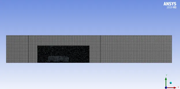
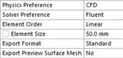
Another body sizing was added to the inner enclosure with element size 25 mm.

Add inflation layer: Similar as the case REFNED MESH 1

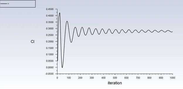
Number of iterations given to run = 1000

Number of iterations to converge = 310

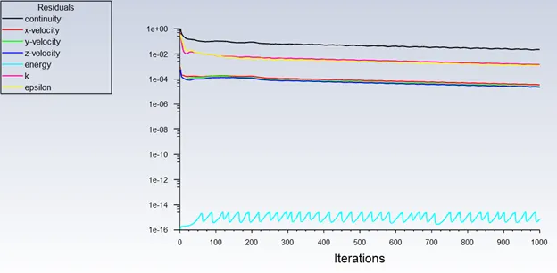
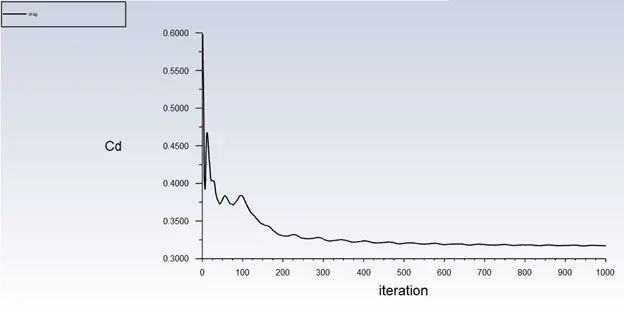
Drag Coefficient = 0.31714585

Lift Coefficient = 0.27620397

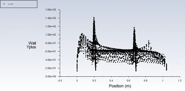
Y⁺ in range for k-epsilon model.

Velocity and Pressure Contour:

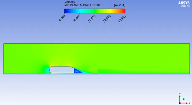
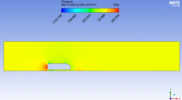
Velocity Vector Plot:

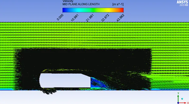
REFINED MESH 3

Similar meshes as REFINED MESH 2 case for both enclosures. Here, the inflation layer will be adjusted to get the accurate results.

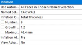
Inflation layer:

Wall spacing = 9 mm

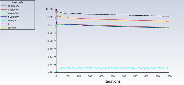
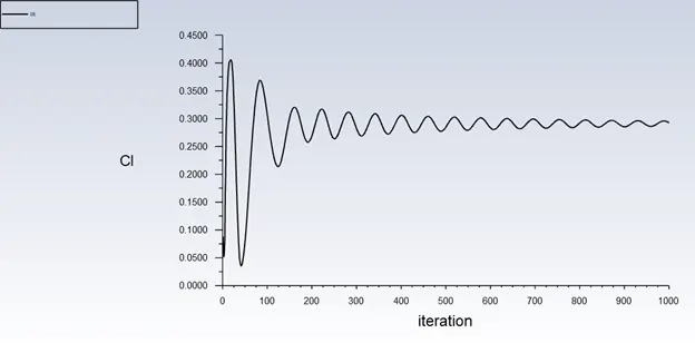
Number of iterations given to run = 1000

Number of iterations to converge = 400

Drag Coefficient = 0.32228175

Lift Coefficient = 0.29264924

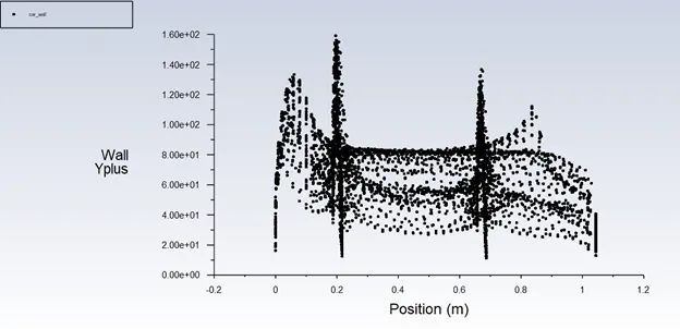
Wall Y⁺ s within the range of the model.

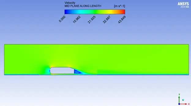
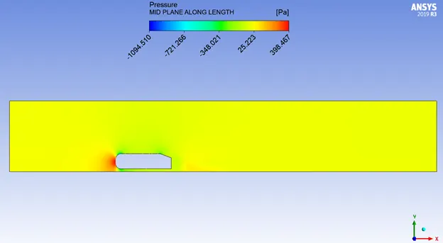
Velocity and Pressure Contour:

Velocity Vector Plot:

REFINED MESH 4

Similar meshes as REFINED MESH 2 case for both enclosures. Here, the inflation layer will be adjusted to get the accurate results.

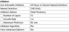
Inflation layer:

Wall spacing = 5 mm

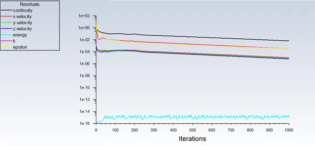
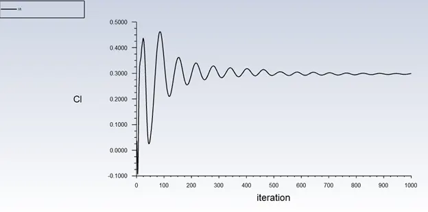
Number of iterations given to run = 1000

Number of iterations to converge = 300

Drag Coefficient = 0.32838728

Lift Coefficient = 0.3087832

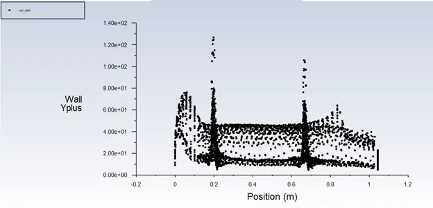
Wall Y⁺ s within the range of the model.

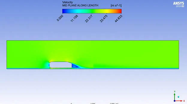
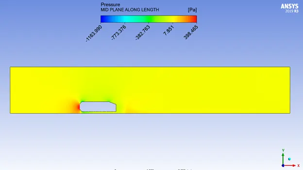
Velocity and Pressure Contour:

Velocity Vector Plot:

INFERENCE:

Cases	Element count	Element size (outer, inner enclosure)	Number of inflation layers	First layer Thickness	Total thickness of inflation layers	Cd
BASELINE MESH	85,165	413.6mm for Both	0	0	0	0.39467476
REFINED MESH 1	178,570	100 mm, 50 mm	5	5 mm	12.5 mm	0.35988549
REFINED MESH 2	1,084,808	50 mm, 25 mm	5	5 mm	12.5 mm	0.31714585
REFINED MESH 3	1,081,021	50 mm, 25 mm	9	9 mm	46.4 mm	0.32228175
REFINED MESH 4	1,103,001	50 mm, 25 mm	15	5 mm	90 mm	0.32838728

As we refined the mesh, we could see the drag coefficient nearing the experimental value of 0.33.

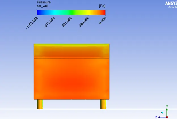
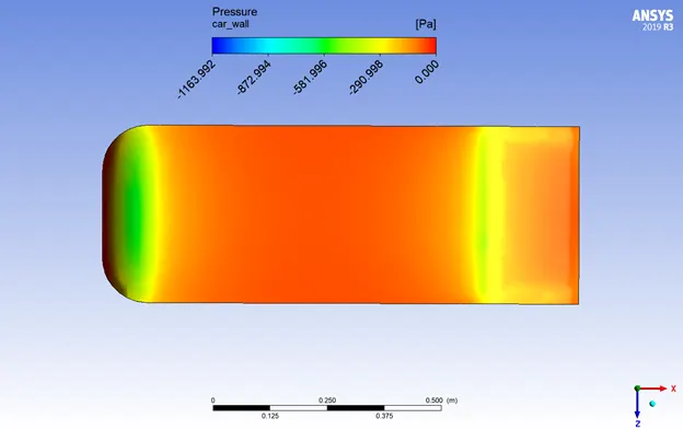
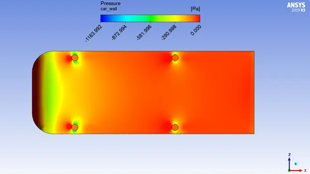
NEGATIVE PRESSURE DISTRIBUTION IN THE WAKE REGION:

NEGATIVE PRESSURE DISTRIBUTION ON THE AHMED BODY:

SIDE VIEW:

FRONT VIEW:

REAR VIEW:

TOP VIEW:

BOTTOM VIEW:

CONCLUSION:

Negative value of pressure here indicates that the pressure fell below the gauge pressure of 0 pa. This is due to the velocity near the wall reduces and the boundary layer thickens. A continuous retardation of flow brings the wall shear stress at the car_wall to zero. From this point onwards the shear stress becomes negative and the flow reverses and a region of recirculating flow develops.

One of the severe effects of an adverse pressure gradient is to separate the flow. The negative pressure gradient will counteract the retarding effect of the shear stress (which is due to viscosity) in the boundary layer. For the geometry considered we have an adverse pressure gradient downstream of the Ahmed body at the wake region.

Now the adverse pressure gradient begins to retard. This effect is felt more strongly in the regions close to the wall where the momentum is lower than in the regions near the free stream. As indicated in the figure, the velocity near the wall reduces and the boundary layer thickens. A continuous retardation of flow brings the wall shear stress at the wall to zero. From this point onwards the shear stress becomes negative and the flow reverses and a region of recirculating flow develops. We see that the flow no longer follows the contour of the body. We say that the flow has separated. The point where the shear stress is zero is called the Point of Separation.