NUMERICAL STUDY OF AERODYNAMICS OF AN AIRFOIL

AIM:

Numerical Study of flow past the classic NACA 0012 airfoil at an angle of attack of 10 degrees.

OBJECTIVE:

1. Comparing the values of Pressure Coefficient (C_P), Coefficient of Lift (C_L) & Coefficient of Drag (C_D) from the numerical study to that of the experimental values.
2. Plotting the velocity and pressure contours in the wake region for further analysis.

NACA 0012 AIRFOIL:

NACA 0012 airfoil Details:

Max thickness - 12% at 30% chord.

Max camber - 0% at 0% chord

Source - UIUC Airfoil Coordinates Database

Dat file:

NACA 0012 AIRFOILS
      66.       66.

 0.0000000 0.0000000
 0.0005839 0.0042603
 0.0023342 0.0084289
 0.0052468 0.0125011
 0.0093149 0.0164706
 0.0145291 0.0203300
 0.0208771 0.0240706
 0.0283441 0.0276827
 0.0369127 0.0311559
 0.0465628 0.0344792
 0.0572720 0.0376414
 0.0690152 0.0406310
 0.0817649 0.0434371
 0.0954915 0.0460489
 0.1101628 0.0484567
 0.1257446 0.0506513
 0.1422005 0.0526251
 0.1594921 0.0543715
 0.1775789 0.0558856
 0.1964187 0.0571640
 0.2159676 0.0582048
 0.2361799 0.0590081
 0.2570083 0.0595755
 0.2784042 0.0599102
 0.3003177 0.0600172
 0.3226976 0.0599028
 0.3454915 0.0595747
 0.3686463 0.0590419
 0.3921079 0.0583145
 0.4158215 0.0574033
 0.4397317 0.0563200
 0.4637826 0.0550769
 0.4879181 0.0536866
 0.5120819 0.0521620
 0.5362174 0.0505161
 0.5602683 0.0487619
 0.5841786 0.0469124
 0.6078921 0.0449802
 0.6313537 0.0429778
 0.6545085 0.0409174
 0.6773025 0.0388109
 0.6996823 0.0366700
 0.7215958 0.0345058
 0.7429917 0.0323294
 0.7638202 0.0301515
 0.7840324 0.0279828
 0.8035813 0.0258337
 0.8224211 0.0237142
 0.8405079 0.0216347
 0.8577995 0.0196051
 0.8742554 0.0176353
 0.8898372 0.0157351
 0.9045085 0.0139143
 0.9182351 0.0121823
 0.9309849 0.0105485
 0.9427280 0.0090217
 0.9534372 0.0076108
 0.9630873 0.0063238
 0.9716559 0.0051685
 0.9791229 0.0041519
 0.9854709 0.0032804
 0.9906850 0.0025595
 0.9947532 0.0019938
 0.9976658 0.0015870
 0.9994161 0.0013419
 1.0000000 0.0012600

 0.0000000 0.0000000
 0.0005839 -.0042603
 0.0023342 -.0084289
 0.0052468 -.0125011
 0.0093149 -.0164706
 0.0145291 -.0203300
 0.0208771 -.0240706
 0.0283441 -.0276827
 0.0369127 -.0311559
 0.0465628 -.0344792
 0.0572720 -.0376414
 0.0690152 -.0406310
 0.0817649 -.0434371
 0.0954915 -.0460489
 0.1101628 -.0484567
 0.1257446 -.0506513
 0.1422005 -.0526251
 0.1594921 -.0543715
 0.1775789 -.0558856
 0.1964187 -.0571640
 0.2159676 -.0582048
 0.2361799 -.0590081
 0.2570083 -.0595755
 0.2784042 -.0599102
 0.3003177 -.0600172
 0.3226976 -.0599028
 0.3454915 -.0595747
 0.3686463 -.0590419
 0.3921079 -.0583145
 0.4158215 -.0574033
 0.4397317 -.0563200
 0.4637826 -.0550769
 0.4879181 -.0536866
 0.5120819 -.0521620
 0.5362174 -.0505161
 0.5602683 -.0487619
 0.5841786 -.0469124
 0.6078921 -.0449802
 0.6313537 -.0429778
 0.6545085 -.0409174
 0.6773025 -.0388109
 0.6996823 -.0366700
 0.7215958 -.0345058
 0.7429917 -.0323294
 0.7638202 -.0301515
 0.7840324 -.0279828
 0.8035813 -.0258337
 0.8224211 -.0237142
 0.8405079 -.0216347
 0.8577995 -.0196051
 0.8742554 -.0176353
 0.8898372 -.0157351
 0.9045085 -.0139143
 0.9182351 -.0121823
 0.9309849 -.0105485
 0.9427280 -.0090217
 0.9534372 -.0076108
 0.9630873 -.0063238
 0.9716559 -.0051685
 0.9791229 -.0041519
 0.9854709 -.0032804
 0.9906850 -.0025595
 0.9947532 -.0019938
 0.9976658 -.0015870
 0.9994161 -.0013419
 1.0000000 -.0012600

FLOW DOMAIN & AIRFOIL MODEL:

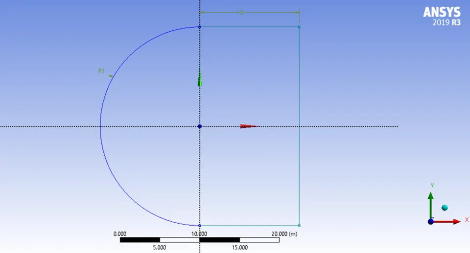
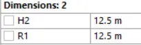
Outer Boundary = 12.5 x c = 12.5 x 1 = 12.5 m (from the airfoil, 12.5 times the chord length)

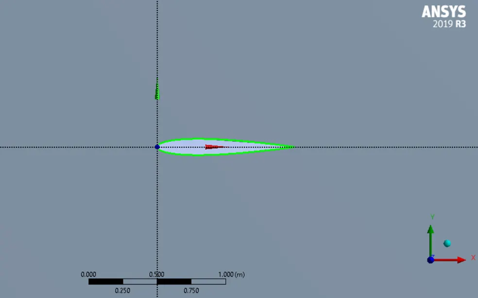
NACA 0012 Airfoil created from the txt file (provided above). A surface was created from the cure that was generated and a Boolean operation was performed on the flow domain.

BOUNDARIES:

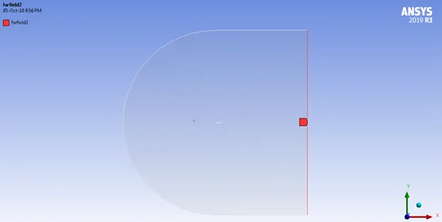
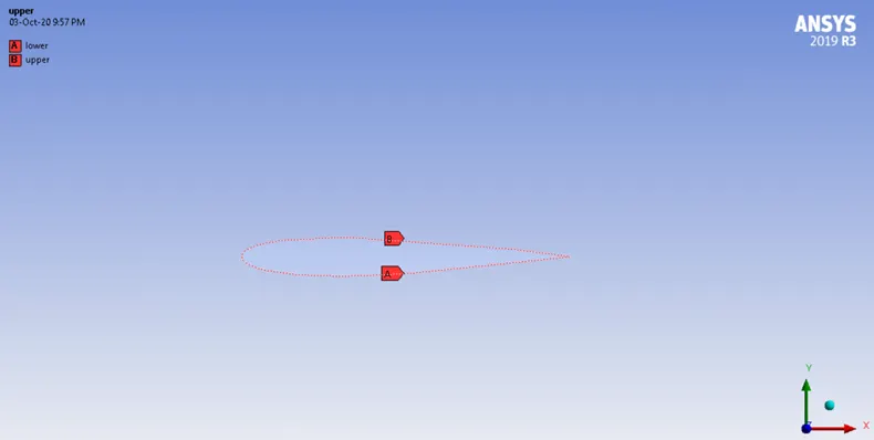
MESH:

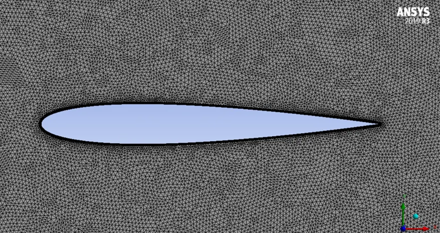
All triangles method applied.

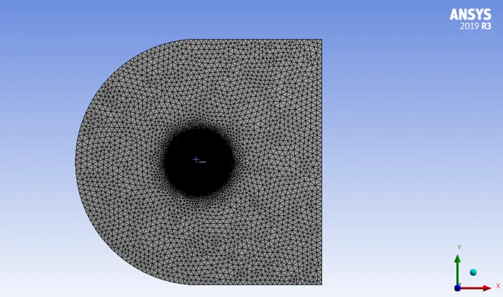
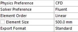
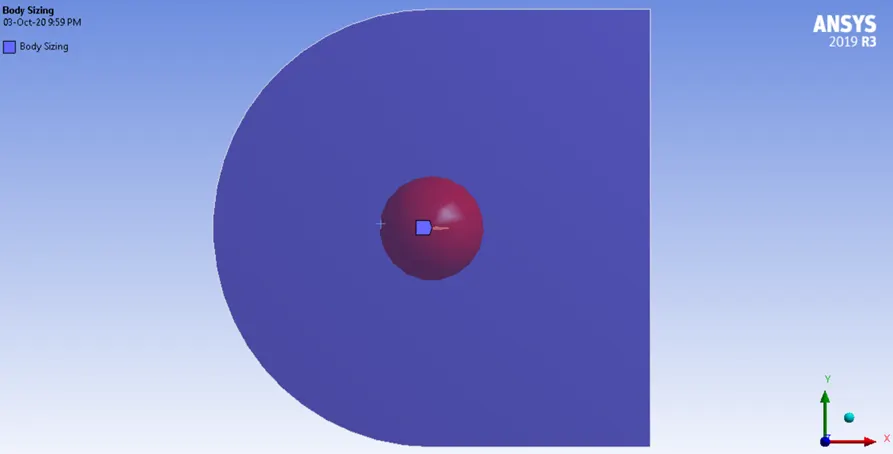
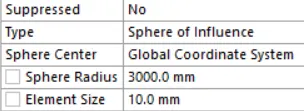
A sphere of influence sizing is applied to the airfoil to better capture the wake region.

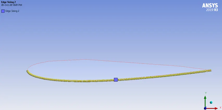
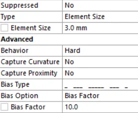
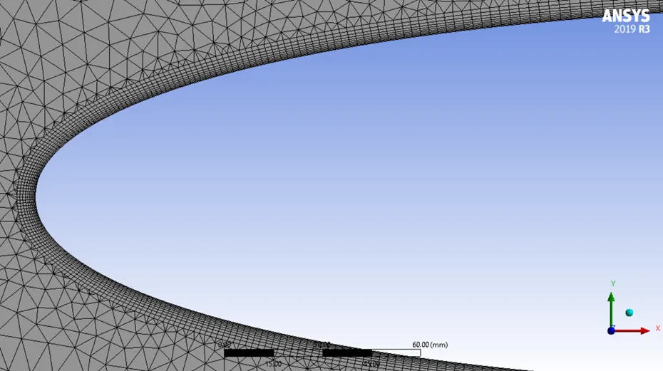
Edge sizing is applied to both lower and upper side of the airfoil. A bias was also given.

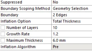
An inflation Layer(s) (10) is also added.

THEORY & SETUP:

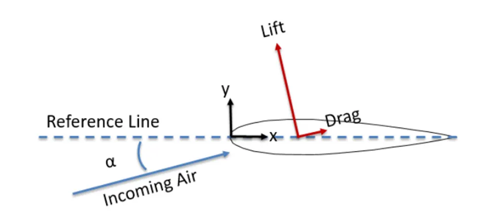
Angle of Attack (a) = 10^o

Airfoil chord length (c) = 1 m

Free-stream velocity (V) = 51.45 m/s

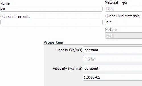
Density (ρ)= 1.1767 kg/m³

Coefficient of viscosity (μ) = 1.009×10^-5 kg/ms

Reynolds Number (Re_C) = `(ρ*V*c)/μ`

Re_C = `(1.1767*51.45*1)/(1.009×10^-5 )` = 6,000,120.41625

Hence, the flow is turbulent. Turbulent K-epsilon Realizable model is used with standard wall treatment is used.

Velocity of Sound = `sqrt((gamma*P)/ρ)` = 349.02 m/s

Mach Number, M = `(Velocity of Air) / (Velocity of Sound)` = `51.45 / 349.02` = 0.148

Since, M < 0.3 pressure-based solver is used.

The material used is air with the following properties:

Creating Definitions:

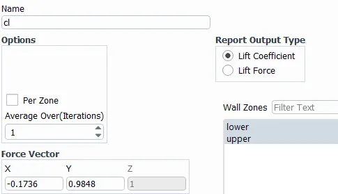
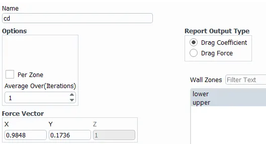
BOUNDARY CONDITIONS:

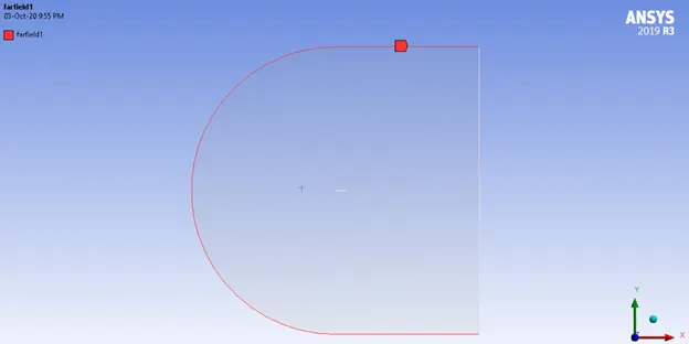
Farfield 1 (Velocity Inlet) `->` u (X velocity) `->` `V*cos(a)` = `51.45*cos(10^o)` = 50.668 m/s

v (Y velocity) `->` `V*sin(a)` = `51.45*sin(10^o)` = 8.934 m/s

Farfield 2 (Pressure Outlet) `->` Gauge pressure = 0 Pa

SIMULATION:

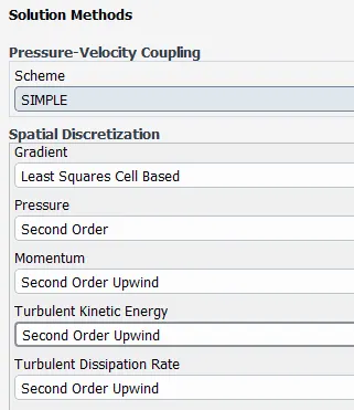
Standard Initialization `->` from farfield 1

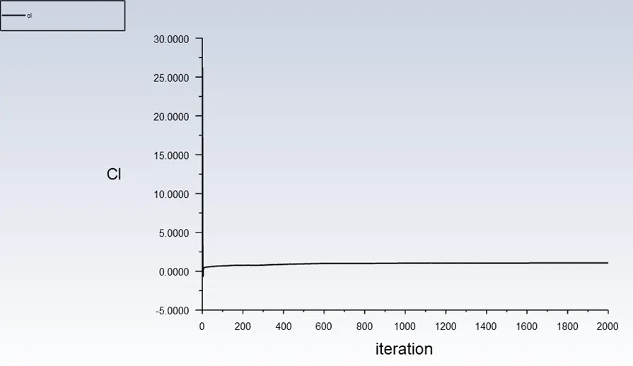
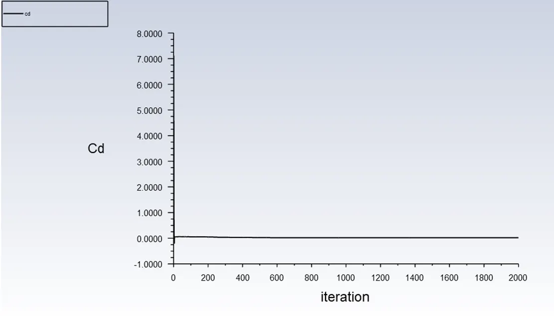
Number of Iterations given to run `->` 2000

Lift Coefficient `->` 1.0596565

Drag Coefficient `->` 0.017423918

OBSERVATIONS:

VELOCITY CONTOUR:

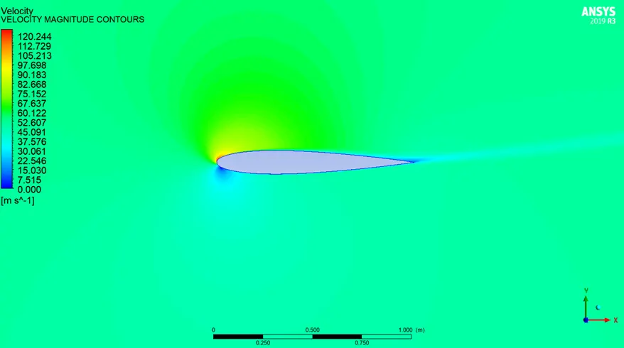
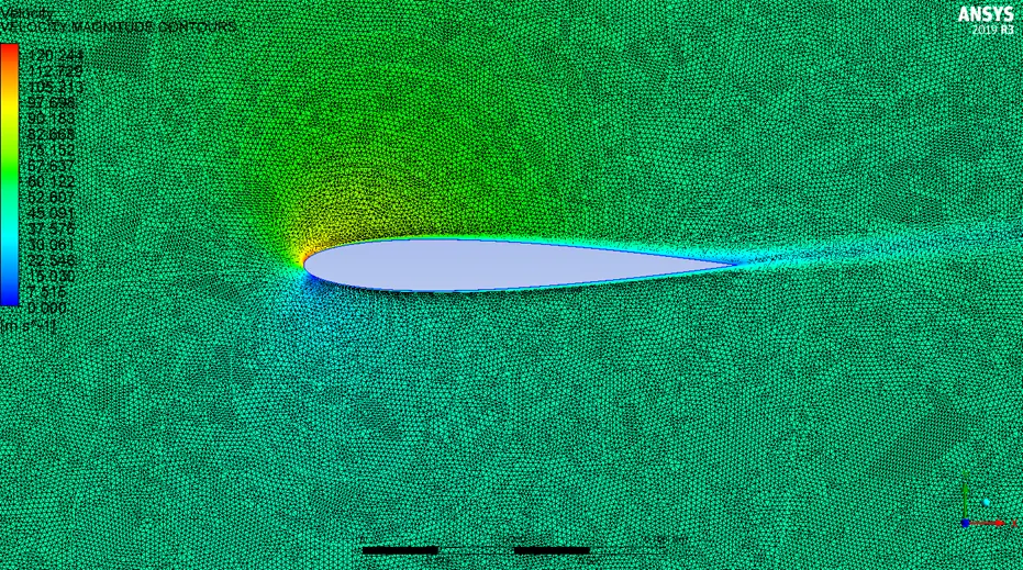
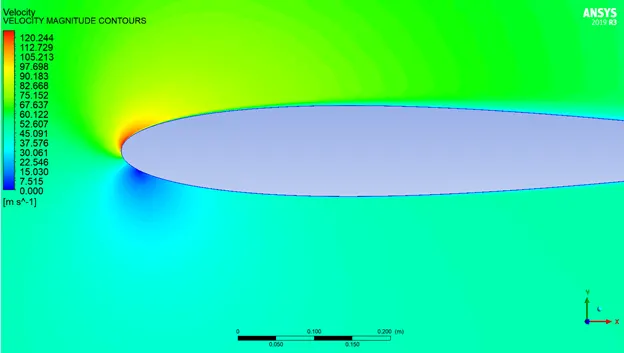
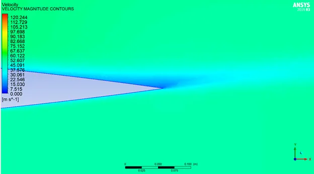
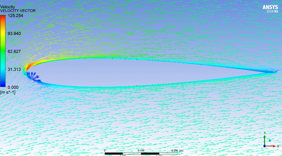
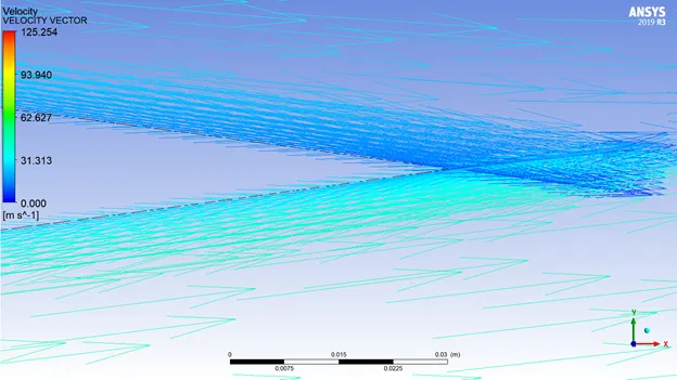
There is a thickening of the turbulent boundary layer as it's coming towards the trailing edge. It's because of the adverse pressure gradient, the net pressure force is pushing the fluid particle back, or it's against the direction of motion. That leads to a thickening of the boundary layer.

PRESSURE CONTOUR:

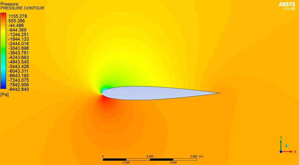
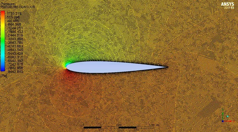
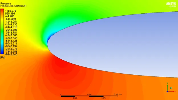
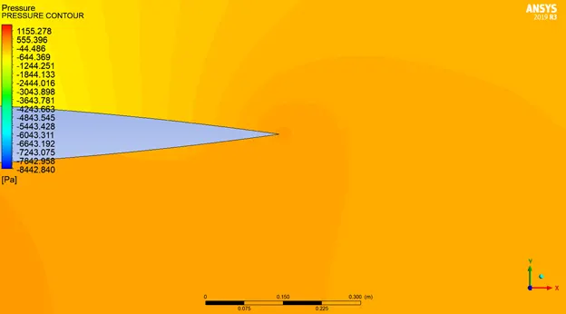
Anytime we have a huge adverse pressure gradient, it causes a thickening of the boundary layer and can also cause separation, as seen at the trailing edge of the airfoil (velocity contour).

VELOCITY VECTOR:

TURBULENT KINETIC ENERGY CONTOUR:

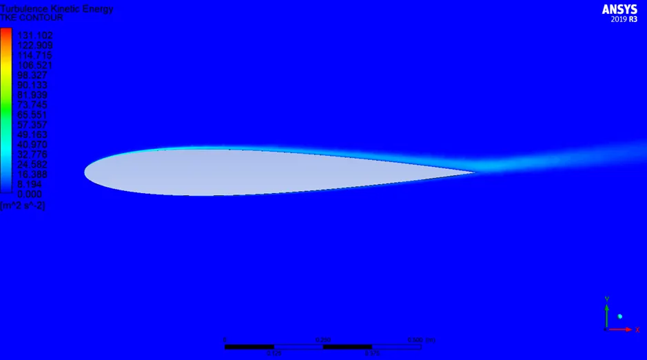
In the adverse pressure gradient region where the flow is slowing down and the boundary layer is thickening, is where most of the turbulence kinetic energy is being generated. And then that's being convected by the flow into the wake.

INFERENCE:

From simulation, Lift Coefficient `->` 1.0596565

From Thin Airfoil Theory (Numerical Hand Calculation):

Lift Coefficient, C_L = `(Li ft)/(ρ*V^2* c *(1))` = 2 (a- a_o) = `2*(pi/180*10 - 0)` = 1.1

The coefficients of lift from the simulation and hand calculations are approximately equal.

Comparring the Pressure Coefficient from simulation to experimental values:

Pressure Coefficient, C_P = `(Gaug e Pressure)/(0.5*ρ*V^2)`

An expression and a variable are created in CFD post. The airfoil is extracted as a polyline to apply the said variable.

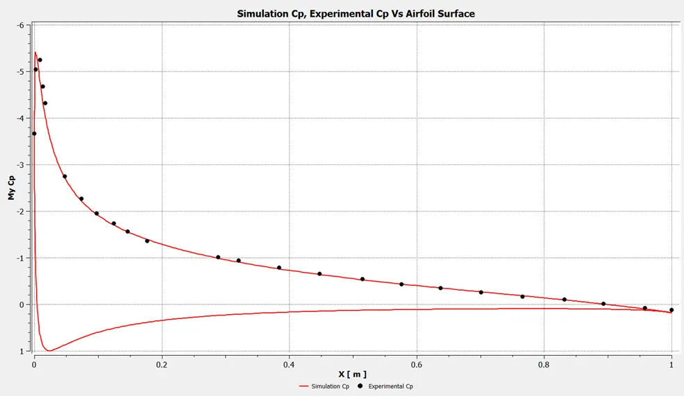
The experimental data is for the upper surface. The pressure coefficient along the airfoil matches quite well with experiment.

Hence the simulation is verified.

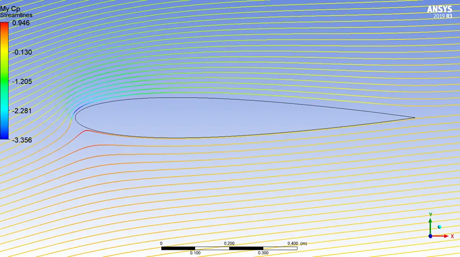
Eulerian View `->` Lagrangian View

CONCLUSION:

1. The simulation was conducted for the angle of attack of 10 degree.
2. The value of Coefficient of Lift (C_L) is compared to the value from the thin airfoil theory and is verified.
3. The value of Pressure coefficients (C_P) from the numerical study is compared to that of the experimental values and is verified along the airfoil upper surface.
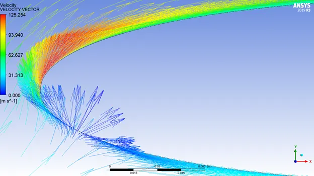
4. The velocity and pressure distribution of the fluid along the leading edge and the trailing edge was analysed and studied, obtaining points of low pressure at the upper leading edge and high pressure at the lower leading edge. The velocity at the upper surface was higher due the the pressure being lower and the vice versa for the lower airfoil surface.