CHT SIMULATION OF AN EXHAUST PORT

Analysis of Conjugate Heat Transfer on an inline four-cylinder, air cooled engine’s exhaust port.

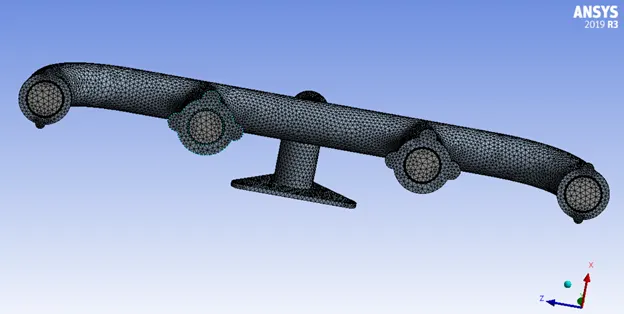
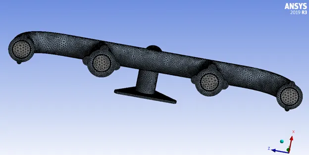
The exhaust port module contains four inlets (which are the outlets for each one of the four cylinders) and one outlet.

OBJECTIVES:

1. Calculation of the wall/surface heat transfer coefficient on the internal solid surface & showing the velocity & temperature contours in appropriate areas.
2. Verification of the Heat Transfer Coefficient (HTC) predictions from the simulations.
3. Ascertain the factors that affect the accuracy of the prediction of Heat Transfer Coefficient.

GOVERNING EQUATION:

INTERNAL & TURBULENT FLOW:

The Dittus-Bölter correlation (1930) is a common and particularly simple correlation useful for many applications. This correlation is applicable when forced convection is the only mode of heat transfer; i.e., there is no boiling, condensation, significant radiation, etc. The accuracy of this correlation is anticipated to be ±15%.

For a fluid flowing in a straight circular pipe with a Reynolds number between 10,000 and 120,000 (in the turbulent pipe flow range), when the fluid's Prandtl number is between 0.7 and 120, for a location far from the pipe entrance (more than 10 pipe diameters; more than 50 diameters according to many authors) or other flow disturbances, and when the pipe surface is hydraulically smooth, the heat transfer coefficient between the bulk of the fluid and the pipe surface can be expressed explicitly as:

`(hd)/k = 0.023*((jd)/μ)^0.8 × ((μ*Cp)/k)^n`

Where,

d is the hydraulic diameter

k is the thermal conductivity of the bulk fluid

μ is the fluid viscosity

j is mass flux

C_p is the isobaric heat capacity of the fluid

n is 0.4 for heating (wall hotter than the bulk fluid) and 0.33 for cooling (wall cooler than the bulk fluid)

The fluid properties necessary for the application of this equation are evaluated at the bulk temperature thus avoiding iteration.

HEAT TRANSFER COEFFICIENT OF PIPE WALL

The resistance to the flow of heat by the material of pipe wall can be expressed as a "heat transfer coefficient of the pipe wall". However, one needs to select if the heat flux is based on the pipe inner or the outer diameter. Selecting to base the heat flux on the pipe inner diameter, and assuming that the pipe wall thickness is small in comparison with the pipe inner diameter, then the heat transfer coefficient for the pipe wall can be calculated as if the wall were not curved

h_wall = `k/x`

where k is the effective thermal conductivity of the wall material and x is the wall thickness.

If the above assumption does not hold, then the wall heat transfer coefficient can be calculated using the following expression:

h_wall = `(2k)/(di*ln((do)/(di)))`

where di and do are the inner and outer diameters of the pipe, respectively.

The thermal conductivity of the tube material usually depends on temperature; the mean thermal conductivity is often used.

CONJUGATE HEAT TRANSFER ANALYSIS:

Conjugate heat transfer (CHT) analysis can accurately predict heat transfer by simultaneous solving all the relevant solid and flow field heat transfer processes, for example: heat exchangers, cooling of electronic equipments, conduction through solids, free and forced convection in the gases/fluids and thermal radiation.

The CHT approach has an advantage over FE thermal analyses in that wall heat transfer coefficients and their local variations on surfaces are directly calculated within the model rather than based on simplified empirical calculations. The CHT approach therefore has benefits for those applications where heat transfer is either non-uniform or difficult to calculate empirically.

EXHAUST PORT MODEL:

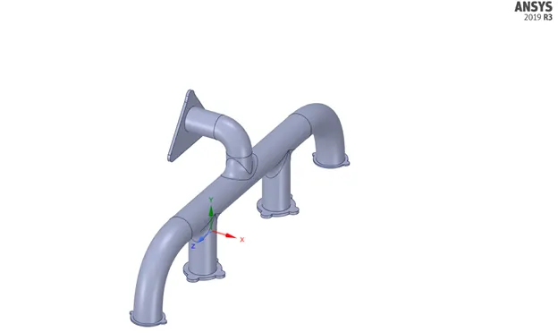
Using ANSYS SpaceClaim the fluid volume was extracted from the model

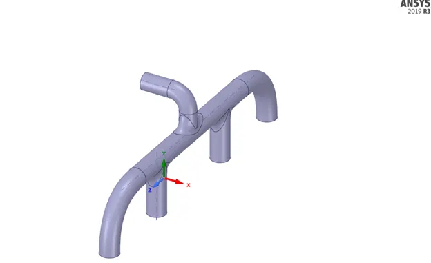
The share topology is set to share.

Using the Share prep in workbench tab of SpaceClaim the coincident topology (interface between the fluid volume and the sold volume) is shared.

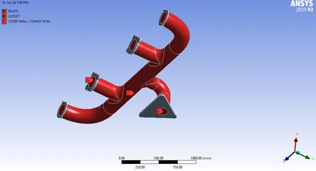
BOUNDARIES:

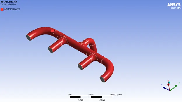
Inflation layer is the outer layer of the fluid volume.

STEADY-STATE SIMULATION:

Materials used: Air (for the fluid volume), Aluminum (for the solid volume) (properties below)

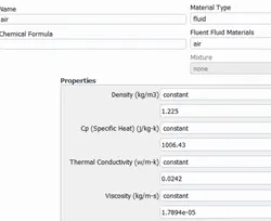
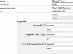
ρ = 1.225 kg/m³

μ = `1.7894 × 10^-5` kg/m-s

d = diameter of the port = 0.166 m

Re_d = `(ρ*V*d)/μ`

V = 5 m/s

Re_d = `(1.225×5× 0.166)/(1.7894 × 10^-5 )` = 56820.72202

Hence, Turbulence Model. Since the wall functions needs to be considered to get wall precise values, k-epsilon model is used in the simulation. With energy equation turned on for conjugate heat transfer analysis.

Solution Method: SIMPLE

Mach Number, M = `(velocity of fluid)/(velocity of sound)`

Velocity of fluid = V = 5 m/s

Velocity of Sound =

𝛄 = 1.4

T = 700 K

Velocity of Sound = 591.7785 m/s

M = `5/591.7785` = 0.0084491072

M < 0.3 (Here, we do not need to take the compressibility factor into account; Incompressible flow)

Hence, Pressure based solver is used.

BOUNDARY CONDITIONS:

INLETS: Velocity Magnitude = 5 m/s

Temperature = 700 K

OUTLET: Pressure (Gauge) = 0 Pa

OUTER WALL CONVECTION: Thermal condition = Convection

Heat Transfer coefficient = 20 W/m²K

BASELINE MESH:

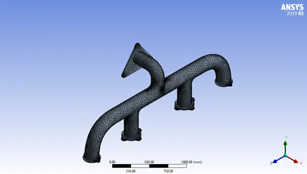
No inflation layers were added to the baseline mesh.

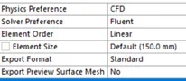
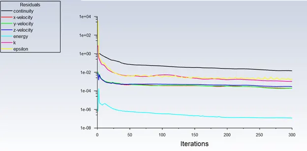
Number of iterations given to run = 300

Number of iterations to converge = 225

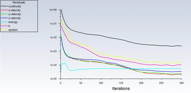
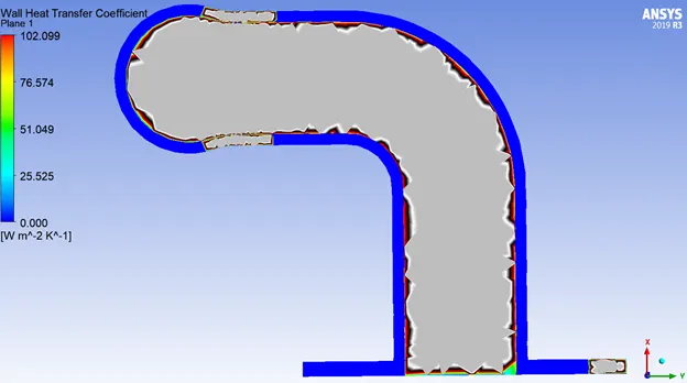
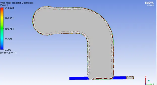
Wall adjacent Heat Transfer Coefficient (inner pipe wall or inflation layer) = 28.181813 W/m²K

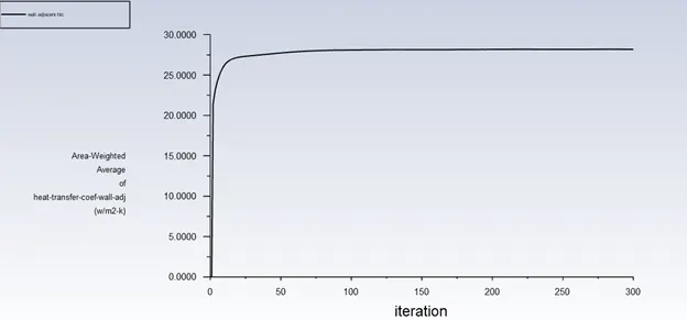
Surface Heat Transfer Coefficient (inner pipe wall or inflation layer) = 21.706514 W/m²K

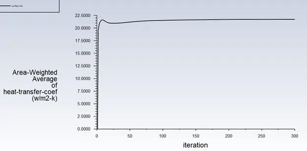
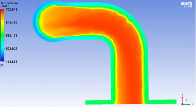
Temperature contour:

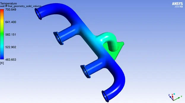
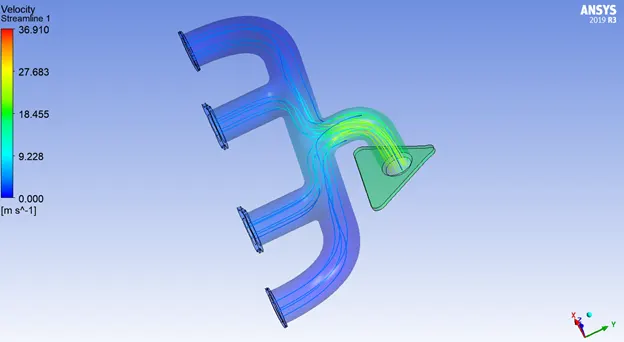
Velocity Streamline:

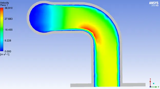
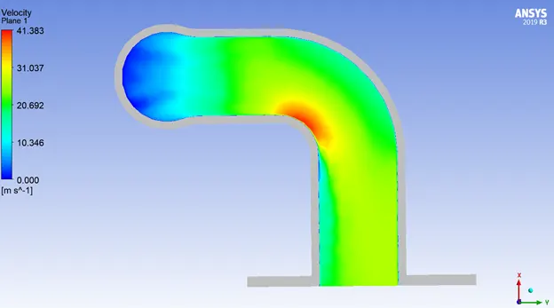
Outlet part contours:

REFINED MESH 1:

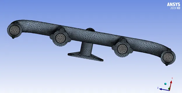
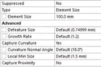
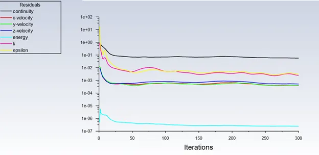
Number of iterations given to run = 300

Number of iterations to converge = 150

Wall adjacent Heat Transfer Coefficient (inner pipe wall or inflation layer) = 83.185572 W/m²K

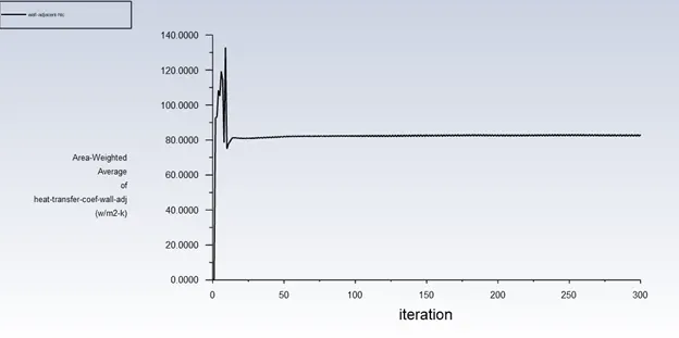
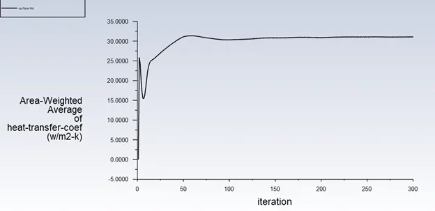
Surface Heat Transfer Coefficient (inner pipe wall or inflation layer) = 31.12744 W/m²K

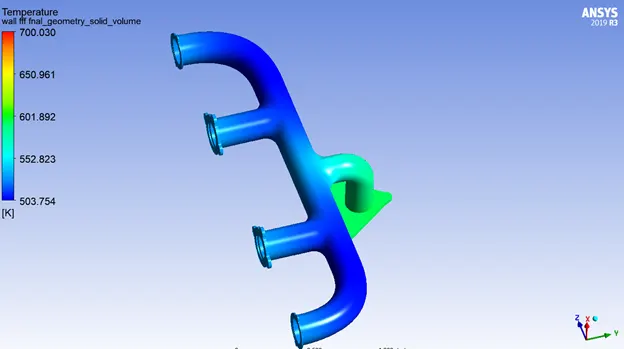
Temperature contour:

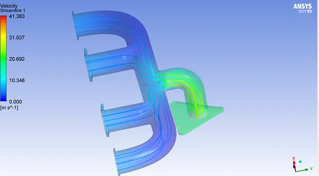
Velocity Streamline:

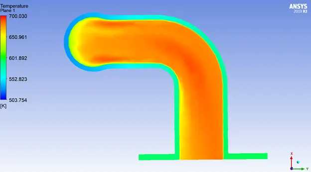
Outlet part contours:

REFINED MESH 2:

Number of iterations given to run = 300

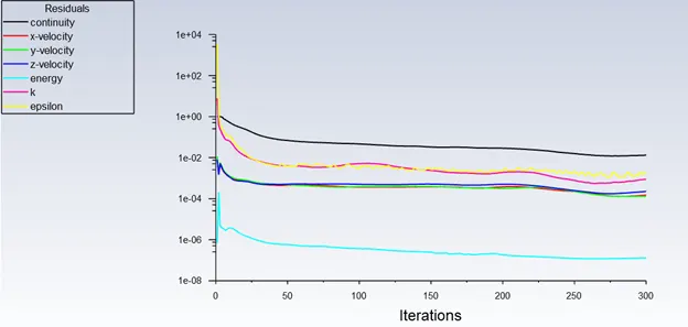
Number of iterations to converge = 100

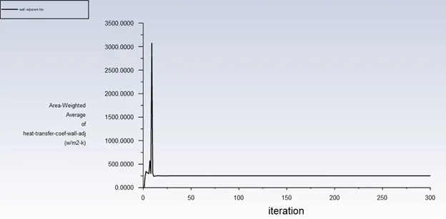
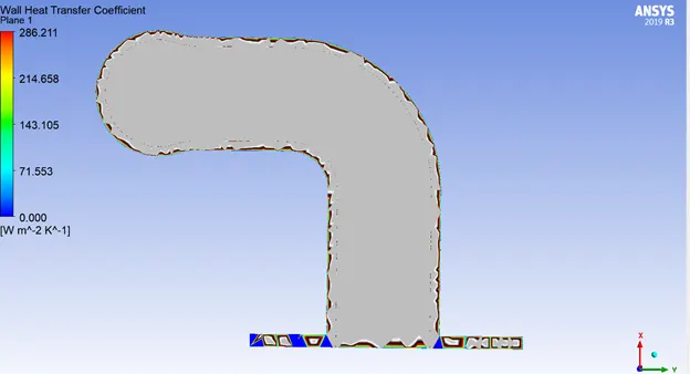
Wall adjacent Heat Transfer Coefficient (inner pipe wall or inflation layer) = 252.14736 W/m²K

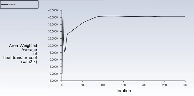
Surface Heat Transfer Coefficient (inner pipe wall or inflation layer) = 40.717037 W/m²K

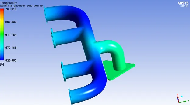
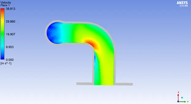
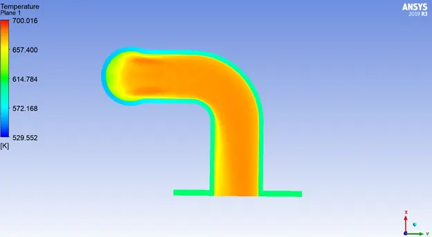
Temperature contour:

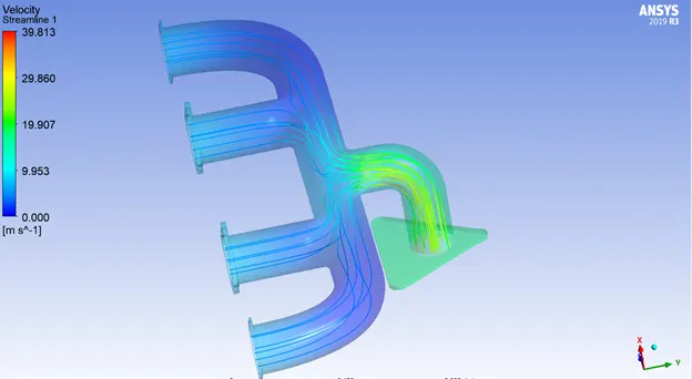
Velocity Streamline:

Outlet part contours:

REFINED MESH 3:

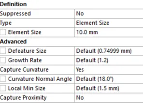
Number of iterations given to run = 300

Number of iterations to converge = 160

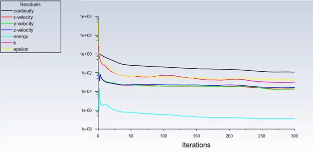
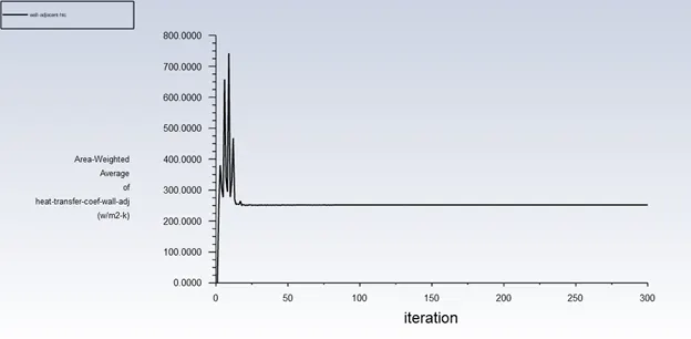
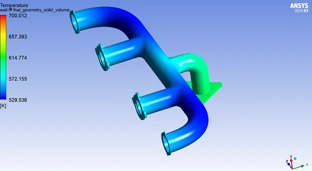
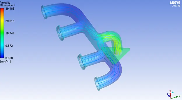
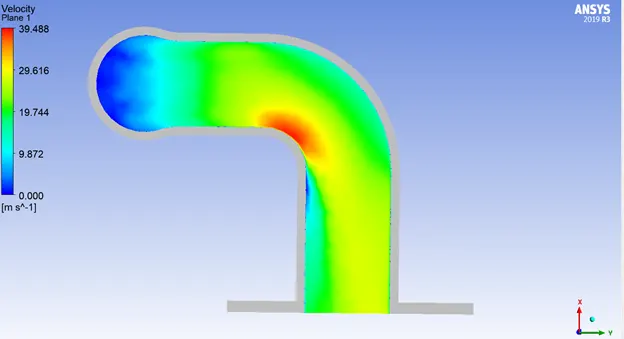
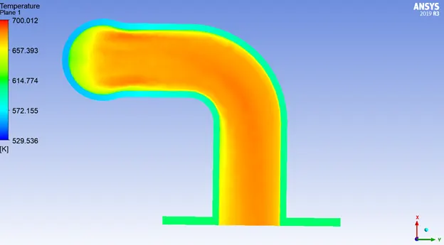
Wall adjacent Heat Transfer Coefficient (inner pipe wall or inflation layer) = 252.13841 W/m²K

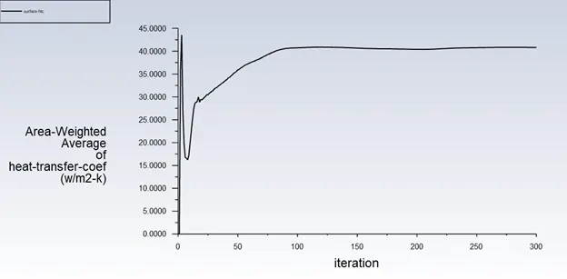
Surface Heat Transfer Coefficient (inner pipe wall or inflation layer) = 40.807518 W/m²K

Temperature contour:

Velocity Streamline:

Outlet part contours:

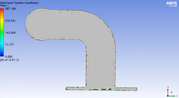
REFINED MESH 4:

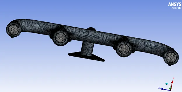
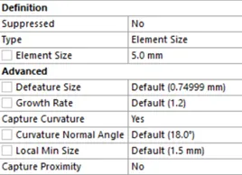
Number of iterations given to run = 300

Number of iterations to converge = 140

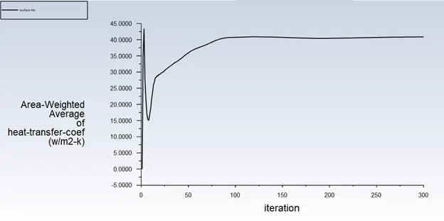
Wall adjacent Heat Transfer Coefficient (inner pipe wall or inflation layer) = 252.13697 W/m²K

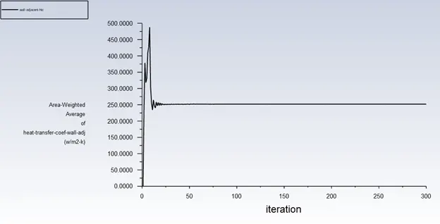
Surface Heat Transfer Coefficient (inner pipe wall or inflation layer) = 40.847211 W/m²K

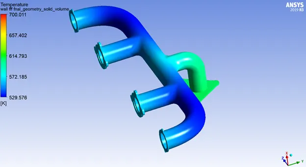
Temperature contour:

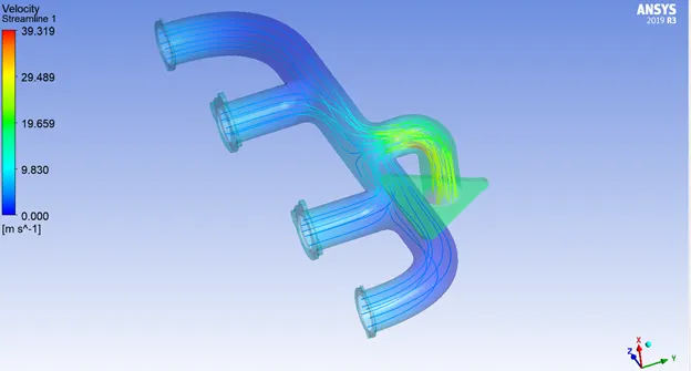
Velocity Streamline:

Outlet part contours:

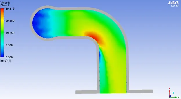
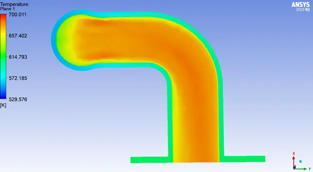
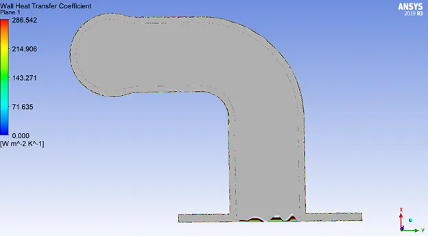
OBSERVATON:

Cases	Element count	Element size	Number of inflation layers	Total thickness of inflation layers	Wall Adjacent Heat Transfer Coefficient (W/m2K)	Surface Feat Transfer Coefficient (W/m2K)
BASELINE MESH	138,496	150 mm	0	5 mm	28.181813	21.706514
REFINED MESH 1	240,810	100 mm	5	5 mm	83.0185572	31.12744
REFINED MESH 2	499,713	20 mm	10	5 mm	252.14736	40.717037
REFINED MESH 3	678,329	10 mm	10	5 mm	252.13841	40.807518
REFINED MESH 4	1,482,218	5 mm	10	5 mm	252.13697	40.847211

INFERENCE:

Through the grid dependency test conducted we can verify the results wall adjacent htc and surface htc. As we move from refined mesh 2 to refined mesh 4 both of those values stop varying.

CONCLUSION:

We can also verify the results by performing hand calculations using the equations of Nusselt Number:

DITTUS-BOELTER EQUATION

The Dittus-Boelter equation (for turbulent flow) is an explicit function for calculating the Nusselt number. It is easy to solve but is less accurate when there is a large temperature difference across the fluid. It is tailored to smooth tubes, so use for rough tubes (most commercial applications) is cautioned. The Dittus-Boelter equation is:

Nu_d = 0.023 Re_d^(4/5) Prⁿ

Where,

d is the inside diameter of the circular duct

Pr is the Prandtl Number

n = 0.4 for fluid being heated, n= 0.3 for fluid being cooled

The Dittus-Boelter equation is valid for

0.6 ≤ Pr ≤ 160

Re_d ≥ 10000

`L/d`≥ 10

And, Nu_d = `(h*d)/k`

The above variables are the factors that the predictions of heat transfer coefficient depend on.

For the simulator the factors such as number of inflation layers, the thickness of inflation layer, number of elements and the grid size affects the accuracy of predictions.