NUMERICAL STUDY OF A CYCLONE SEPARATOR

AIM:

To perform analysis on cyclone separator and calculate the separation efficiency and pressure drop.

OBJECTIVE:

1. Four empirical models used to calculate the cyclone separator efficiency.
2. To perform an analysis on a given cyclone separator model by varying the particle diameter from 1 μm to 5 μm and to calculate the separation efficiency in each case. [Both velocities are 3m/sec.]
3. To perform an analysis on a given cyclone separator model by varying the particle velocity from 1 m/sec to 5 m/sec and calculating the separation efficiency and pressure drop in each case. [Particle diameter size is 5 μm for all cases & keeping flow velocity same as particle velocity]

GOVERNING EQUATIONS:

There are three models commonly used in cyclone simulation: k–e model, algebraic stress model (ASM) and RSM. The k–epsilon model adopts the assumption of isotropic turbulence, so it is not suitable for the flow in a cyclone which has anisotropic turbulence. ASM cannot predict the recirculation zone and Rankine vortex in strongly swirling flow. RSM forgoes the assumption of isotropic turbulence and solves a transport equation for each component of the Reynolds stress. It is regarded as the most applicable turbulent model for cyclone flow even though it has the disadvantage of being computationally more expensive. In the RSM, the transport equation is written as:

Where the left two terms are the local time derivative of stress and convective transport term, respectively. The right five terms are:

Stress diffusion term:

Shear production term: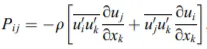

Pressure-strain term: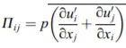

Dissipation term: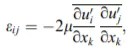

Source term: S

CYCLONE SEPERATORS:

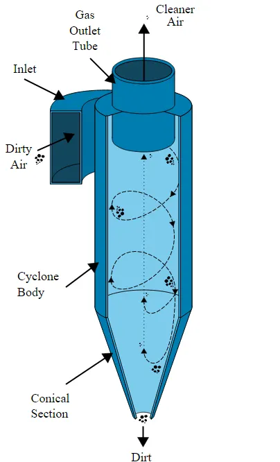
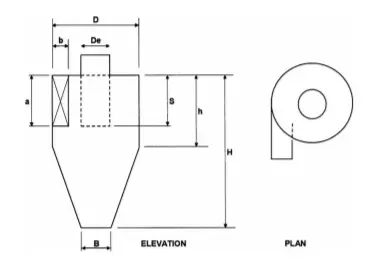
Cyclones are devices that employ a centrifugal force generated by a spinning gas stream to separate particles from the carrier gas. Their simple design, low capital cost and nearly maintenance-free operation make them ideal for use as precleaners for more expensive final control devices such as bag30 houses or electrostatic precipitators. Cyclones are particularly well suited for high temperature and pressure conditions because of their rugged design and flexible component materials. Cyclone collection efficiencies can reach 99% for particles bigger than 5 µm.

Gas cyclone separator is widely used in industries to separate dust from gas or for product recovery because of its geometrical simplicity, relative economy in power and flexibility. The conventional method of predicting the flow field and the collection efficiency of a cyclone is empirical. In the past decade, application of computational fluid dynamics (CFD) for the numerical calculation of the gas flow field becomes more and more popular. One of the first CFD simulations was done by Boysan.

Many different types of cyclones have been built but the reverse flow cyclone with tangential inlet is most often used for industrial gas cleaning. In this study, the numerical simulation deals with the standard case of reverse flow cyclone with a tangential rectangular inlet.

Collection efficiency statistics were obtained by releasing a specified number of monodispersed particles at the inlet of the cyclone and by monitoring the number escaping through the underflow, i.e. Here, ratio of total number of particles trapped to the total number of particles tracked.

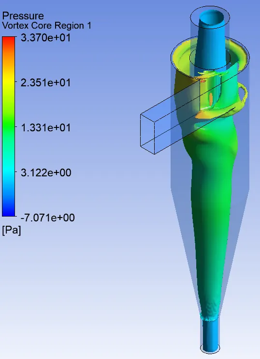
Pressure drop is defined as the pressure difference between two points. i.e. Here, difference between Total inlet pressure and Total outlet pressure (OUTLET 1-TOP).

CYCLONE EFFICIENCY EMPIRICAL MODELS:

IOZIA AND LEITH MODEL:

Iozia and Leith logistic model is a modified version of Barth Model, which is developed based on force balance. The model assumes that a particle carried by the vortex endures the influence of two forces: a centrifugal force, Z and a flow resistance, W. The collection efficiency η_i of particle diameter d_pi can be calculated from

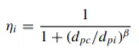
β is an expression for slope parameter derived based on the statistical analysis of experimental data of a cyclone with D = 0.25 m given as

LI AND WANG MODEL:

The Li and Wang model includes particle bounce or reentrainment and turbulent diffusion at the cyclone wall. A two-dimensional analytical expression of particle distribution in the cyclone is obtained. Li and Wang model was developed based on the following assumptions:

• The radial particle velocity and the radial concentration profile are not constant for uncollected particles within the cyclone.
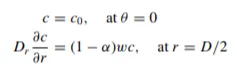
• Boundary conditions with the consideration of turbulent diffusion coefficient and particle bounce reentrainment on the cyclone wall are:

• The tangential velocity is related to the radius of cyclone by: u Rⁿ = constant.

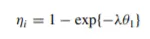
KOCH AND LICHT MODEL:

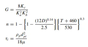
Koch and Licht collection theory recognized the inherently turbulent nature of cyclones and the distribution of gas residence times within the cyclone. Koch and Licht described particle motion in the entry and collection regions with the additional following assumptions:

• The tangential velocity of a particle is equal to the tangential velocity of the gas flow, i.e. there is no slip in the tangential direction between the particle and the gas.
• The tangential velocity is related to the radius of cyclone by: u Rⁿ = constant.

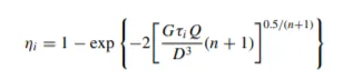
A force balance and an equation on the particles collection yields the grade efficiency η_i

LAPPLE MODEL:

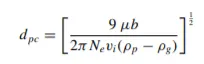
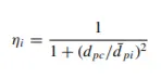
Lapple model was developed based on force balance without considering the flow resistance. Lapple assumed that a particle entering the cyclone is evenly distributed across the inlet opening. The particle that travels from inlet half width to the wall in the cyclone is collected with 50% efficiency. The semi empirical relationship developed by Lapple to calculate a 50% cut diameter, d_pc, is

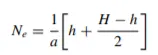
The efficiency of collection of any size of particle is given by

MODEL AND FLOW DOMAIN:

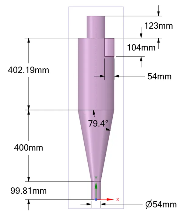
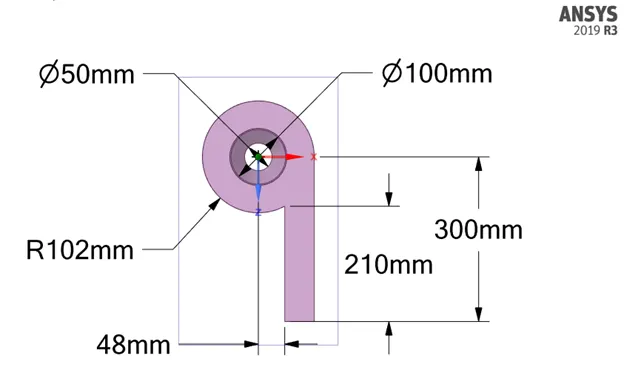
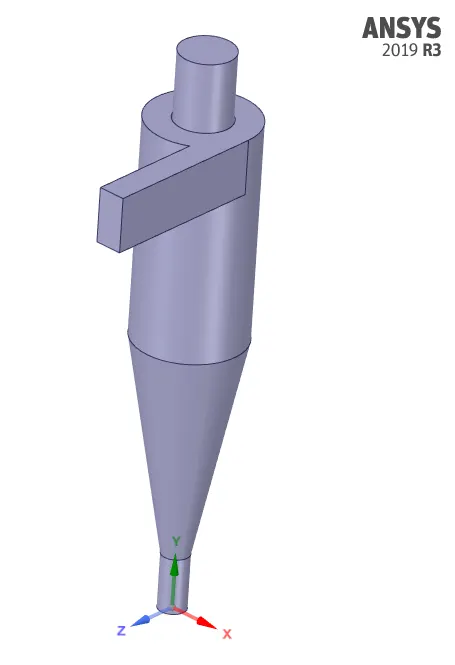
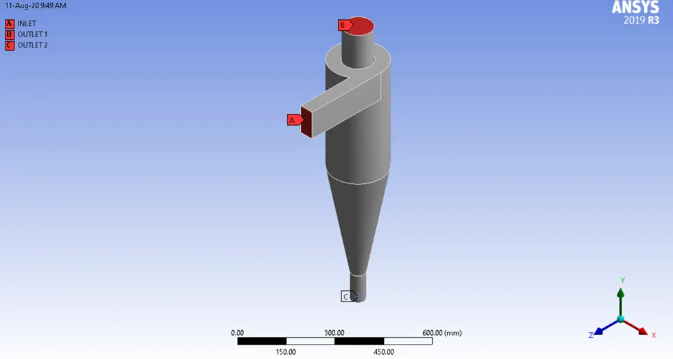
Gas cyclone seperator model was prepared in ANSYS SpaceClaim with the following dimensions.

The fluid volume was prepared using Volume Extract

BOUNDARIES:

MESH:

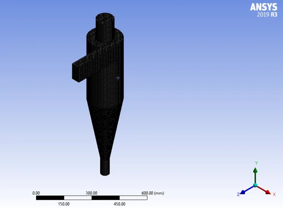
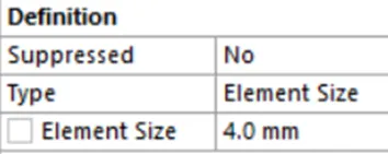
Structural mesh gives the best results, so cutcell meshing approach available in Ansys Meshing used with body sizing.

STEADY-STATE SIMULATION SETUP:

To reduce the computational effort, the RNG k-epsilon model can be used with about 12% deviation on experimental data. RNG k-epsilon model underestimates the variation of the axial velocity profile across the radial direction and also overestimates the magnitude of the tangential velocity and the cyclone pressure drop.

The finite volume method has been used to discretize the partial differential equations of the model using the SIMPLE method for pressure-velocity coupling and the Second Order Upwind scheme to interpolate the variables on the surface of the control volume.

RNG K-epsilon Model:

Good for moderately complex behavior like jet impingement, separating flows, swirling flows, and secondary flows. Subjected to limitations due to isotropic eddy viscosity assumption.

Pressure based solver

Gravity `->` y = -9.81 m/s²

Turbulence Model `->` Reynolds stress model (RSM) RNG k-epsilon `->` Swirl Dominated Flow

Continuous Phase `->` Air

Discretization:

Pressure-Velocity Coupling `->` SIMPLE

Momentum `->` 2^nd Order Upwind

Turbulence Kinetic Energy `->` 2^nd Order Upwind

Turbulence Dissipation Rate `->` 2^nd Order Upwind

Reynolds Stresses `->` 2^nd Order Upwind

Discrete Phase Modelling:

Assumption `->` Spherical Particle

Injection `->` Surface `->` INLET

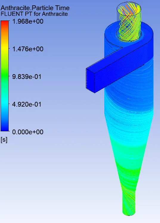
Injection Material `->` Anthracite (Uniform Diameter)

Maximum Number of Steps (Phase Integration) `->` 500000

DPM BOUNDARY CONDITIONS:

INLET & WALL `->` Reflect

OUTLET 1 (TOP) `->` Escape

OUTLET 2 (BOTTOM/DUSTBIN) `->` Trap

SIMULATIONS WITH VARYING PARTCLE DIAMETER

Velocity of Discrete and Continuous Phase = 3 m/s (constant for all cases)

CONTINUOUS PHASE `->` Fluid (Air) Flow

DISCRETE PHASE `->` Anthracite Particle

Standard Initialization from INLET

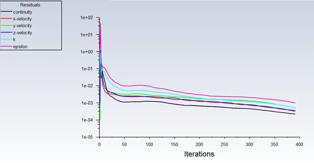
Number of Iterations given to run = 600

Number of Iterations to Converge = 391 (for all cases)

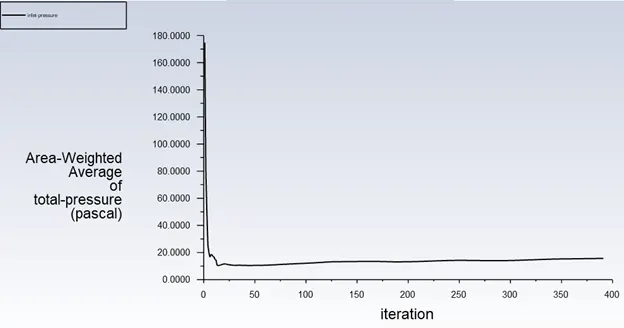
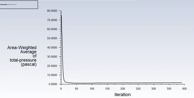
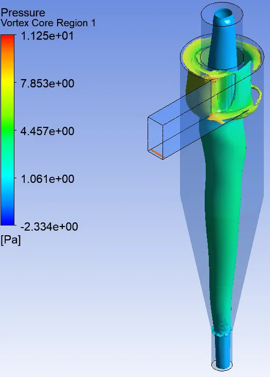
Inlet Pressure = 15.68021 Pa, Outlet (Top) Pressure = 1.6792029 Pa

Particle Diameter = 1 μm

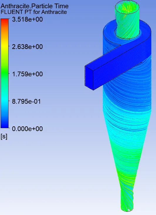
Particle Diameter = 2 μm

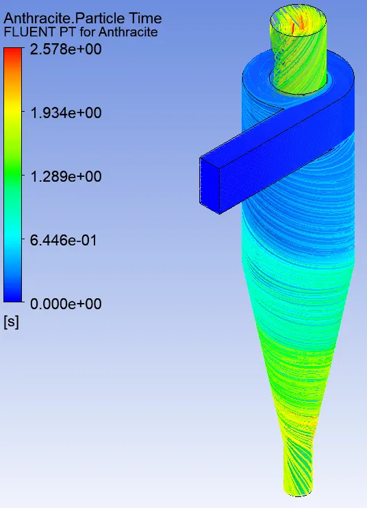
Particle Diameter = 3 μm

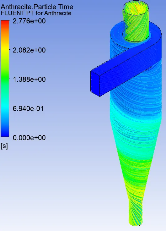
Particle Diameter = 4 μm

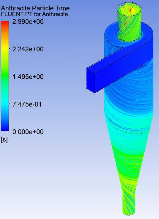
Particle Diameter = 5 μm

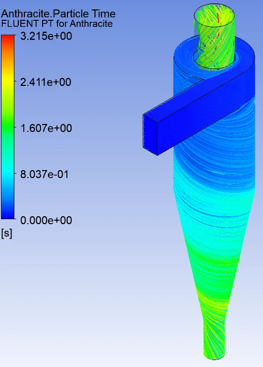
SIMULATIONS WITH VARYING VELOCITY (FLOW/CONTINUOUS PHASE & PARTICLE/DISCRETE PHASE)

Discrete Phase Particle Diameter = 5 μm (constant for all cases)

CONTINUOUS PHASE `->` Fluid (Air) Flow

DISCRETE PHASE `->` Anthracite Particle

Standard Initialization from INLET

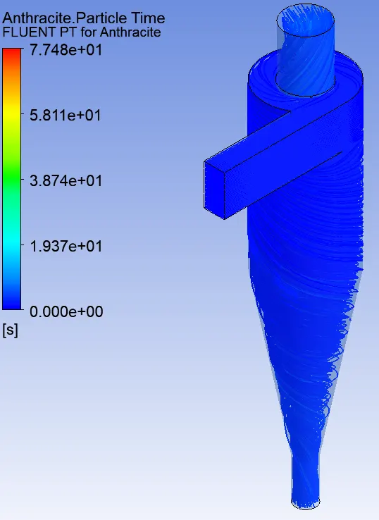
Flow/Continuous Phase & Particle/Discrete Phase Velocity = 1 m/s

Number of Iterations given to run = 600

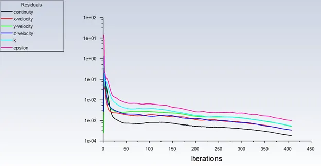
Number of Iterations to Converge = 408

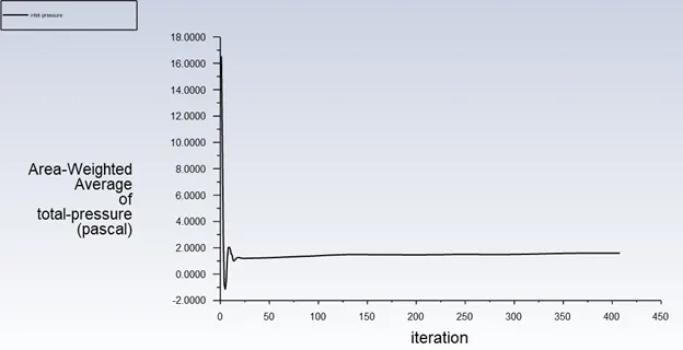
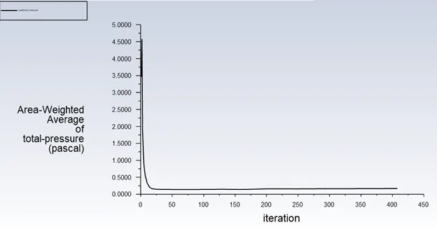
Inlet Pressure = 1.6008828 Pa, Outlet (Top) Pressure = 0.16994228 Pa

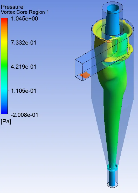
Flow/Continuous Phase & Particle/Discrete Phase Velocity = 2 m/s

Number of Iterations given to run = 600

Number of Iterations to Converge = 396

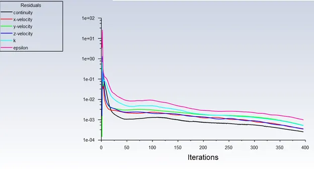
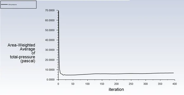
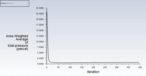
Inlet Pressure = 6.762334 Pa, Outlet (Top) Pressure = 0.7159392 Pa

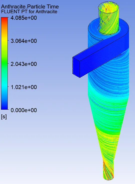
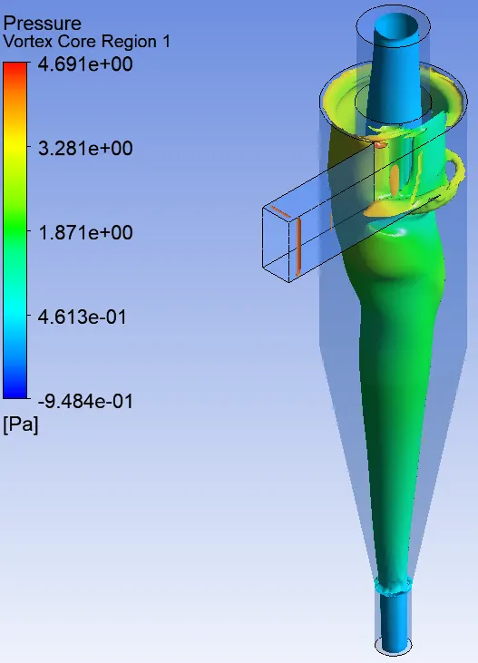
Flow/Continuous Phase & Particle/Discrete Phase Velocity = 4 m/s

Number of Iterations given to run = 600

Number of Iterations to Converge = 392

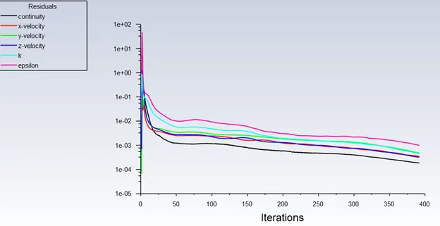
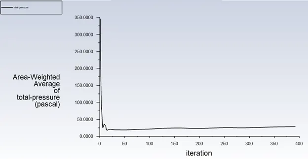
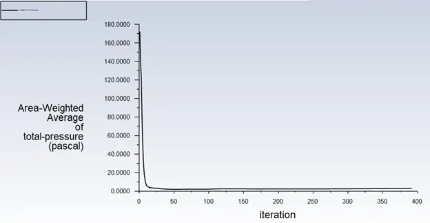
Inlet Pressure = 28.532811 Pa, Outlet (Top) Pressure = 3.0840489 Pa

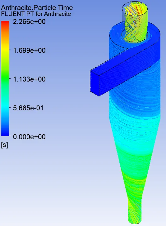
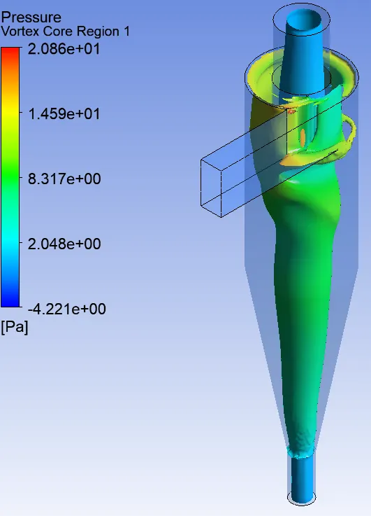
Flow/Continuous Phase & Particle/Discrete Phase Velocity = 5 m/s

Number of Iterations given to run = 600

Number of Iterations to Converge = 399

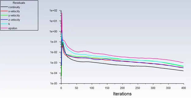
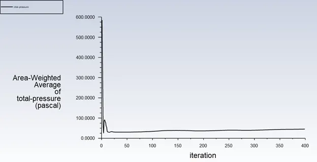
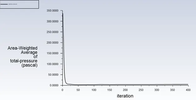
Inlet Pressure = 45.472526 Pa, Outlet (Top) Pressure = 4.9719054 Pa

OBSERVATONS:

SIMULATIONS WITH VARYING PARTCLE DIAMETER:

Inlet Pressure = 15.68021 Pa

Outlet (Top) Pressure = 1.6792029 Pa

Pressure Drop = 14.001007 Pa

Particle Size (μm)	Flow (Continuous Phase) Velocity (m/s)	Particle (Discrete Phase) Velocity (m/s)	Particles Tracked	Particles Escaped	Particles Trapped	Particles Incomplete	Efficiency (%)
1	3	3	465	236	226	3	48.6021
2	3	3	465	225	240	0	51.6129
3	3	3	465	203	262	0	56.344
4	3	3	465	177	288	0	61.935
5	3	3	465	146	319	0	68.6021

SIMULATIONS WITH VARYING VELOCITY (FLOW/CONTINUOUS PHASE & PARTICLE/DISCRETE PHASE):

Particle Size (μm)	Flow (Continuous Phase) Velocity (m/s)	Particle (Discrete Phase) Velocity (m/s)	Particles Tracked	Particles Escaped	Particles Trapped	Particles Incomplete	Efficiency (%)	Inlet Pressure (Pa)	Outlet (Top) Pressure (Pa)	Pressure Drop (Pa)
5	1	1	465	233	117	115	25.1612	1.6008828	0.169942	1.4309408
5	2	2	465	186	279	0	60.0	6.762334	0.7159392	6.046404
5	3	3	465	146	319	0	68.6021	15.68021	1.6792029	14.001007
5	4	4	465	105	360	0	77.4193	28.5381	3.0840489	25.4540511
5	5	5	465	65	400	0	86.0215	45.472526	4.9719054	40.5006206

INFERENCE:

For Constant Velocity of Discrete and Continuous Phase (3 m/s):

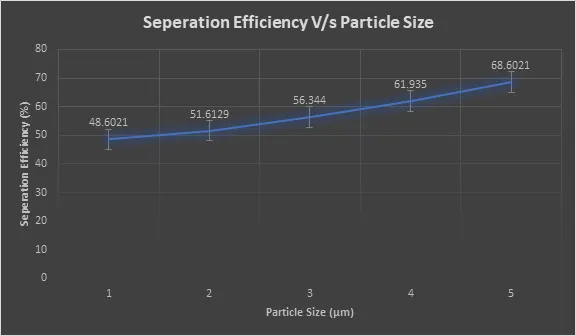
Seperaton efficiency increases as the particle size increases.

For Constant Discrete Phase Particle Diameter (5 μm):

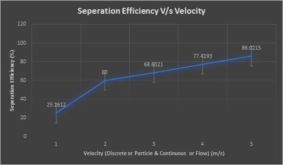
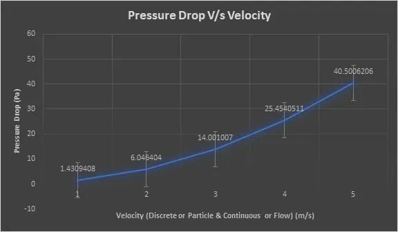
Seperation efficiency and pressure drop increases as the velocity increases.

CONCLUSION:

• From the plot of separation efficiency v/s particle size we can see that the separation efficiency rises as the particle size increases for the constant velocity of 3 m/s (for both the discrete and continuous phase). This is due the reduction of incomplete particles and particles escaped. As the particle size increases the number of particles escaped reduces since more particles are getting trapped, hence the increase in efficiency (Ratio of No: of Particles trapped to the Number of particles tracked).
• From the plot of separation efficiency v/s velocity (with constant particle size of 5 μm) we can observe that the efficiency increases as the velocity increases. Since the mass flow rate increases more particles are getting trapped, hence the increase in efficiency.
• Variation in pressure drop is observed when there is a variation in velocity and not observed when there is a variation in particle size with velocity being constant.
• Separation efficiency of a cyclone separator depends on both velocity and particle size as seen by these plots of variations. But, separation efficiency is largely affected by velocity rather than particle size, since the variation observed with velocity is higher than the variation observed with particle size.