Week 8: Literature review - RANS derivation and analysis
Aim: Literature review - RANS derivation and analysis
Objective:
Apply Reynolds decomposition to the NS equations and come up with the expression for Reynolds stress.
- Explain your understanding of the terms Reynolds stress
- What is turbulent viscosity? How is it different from molecular viscosity?
Introduction
In fluid dynamics, the Reynolds Stress is the component of the total stress tensor in a fluid obtained from the averaging operation over the Navier-Stokes equations to account for turbulent fluctuations in the fluid momentum.
Reynolds suggested that there are velocity fluctuations present in the flow that can split the velocity term into two parts, one the mean velocity and the other the fluctuation over the mean velocity. The convective momentum transport can now have two (or more) parts. First, is the convective momentum transport due to the mean velocity of the flow and the particles. The second one (which is, technically, the Reynolds stress term) is the momentum transfer due to the fluctuations in the velocities. To put it simply it is the mean transport of the fluctuating momentum by turbulent velocity fluctuations. This term, therefore, complements fluid viscosity in the transport of momentum, but convectively.
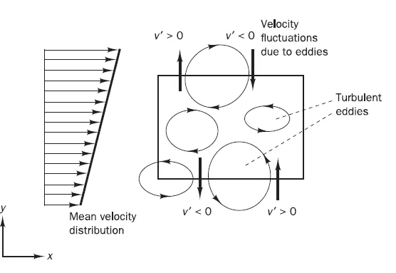
Fig: Control volume within a two-dimensional turbulent shear flow
Reynolds-averaged Navier---Stokes equations for incompressible flow
The consequences of turbulent fluctuations for the mean flow equations for an incompressible flow with constant viscosity. The rules which govern time averages of fluctuating properties ϕ = Φ +ϕ′ and ψ = Ψ +ψ′ and their summation, derivatives, and integrals.
Equation 1
`barphi^'=baromega^'=0`
`barPhi=Phi`
`frac{bar(delphi)}{dels}=frac{delPhi}{dels}`
`intbar(phids)=intPhids`
`bar(phi+omega)=Phi+Psi`
`bar(phiomega)=PhiPsi+bar(phi^'omega^')`
`bar(phiPsi)=PhiPsi`
`bar(phi^'Psi)=0`
It can be concluded that the time-averaging operation is itself an integration. Thus, the order of time-averaging and summation, further integration, and/or differentiation can be swapped or commuted, so this is called the commutative property.
Since div and grad are both differentiations, the above rules can be extended to a fluctuating vector quantity a = A + a′ and its combinations with a fluctuating scalar ϕ = Φ +ϕ ′:
Equation 2
`bar(d iva)=d iv A`
`bar(d iv(phia))=d iv(bar(phia))=d iv(Phia)+d iv(bar(phi^'a^'));`
`bar(d iv gr adphi)=d ivg radPhi`
The instantaneous continuity and Navier–Stokes equations are considered in a Cartesian coordinate system so that the velocity vector u has x-component u, y-component v, and z-component w:
Equation 3
`d ivu=0`
`frac{delu}{delt}+d iv(u u)=frac{-1}{rho}frac{delrho}{delx}+vd iv(gr ad(u))`
`frac{delv}{delt}+d iv(vu)=frac{-1}{rho}frac{delrho}{dely}+vd iv(gr ad(v))`
`frac{delw}{delt}+d iv(wu)=frac{-1}{rho}frac{delrho}{delz}+vd iv(gr ad(w))`
This system of equations governs every turbulent flow, but the effects of fluctuations are investigated on the mean flow using the Reynolds decomposition and replace the flow variables u (hence also u, v, and w) and p by the sum of a mean and fluctuating component.
Thus u = U + u′ u = U + u′ v = V + v′ w = W + w′ p = P + p′
Then the time average is taken, from equation 3, first we note that `bar(d ivu)`= div U. This yields the continuity equation for the mean flow:
div U = 0
A similar process is now carried out on the x-momentum equation. The time averages of the individual terms in this equation can be written as follows:
Equation 4
`frac{bar(delu)}{delt}=frac{delU}{delt}`
`bar(d iv(u u))=d iv(U U)+d ivbar(u^'u^')`
`bar(frac{-1}{rho}frac{delp}{delx})=frac{-1}{rho}frac{delP}{delx}`
`bar(vd iv(gr ad(u)))=vd iv(gr ad(U))`
The time-average x-momentum equation is given by
Equation 5
`frac{delU}{delt}+ d iv(UU)+d iv(bar(u^'u^'))=frac{-1}{rho}frac{delP}{delx}+vd iv(g rad(U))`
The time-average y-momentum equation is given by
Equation 6
`frac{delV}{delt}+ d iv(VU)+d iv(bar(v^'u^'))=frac{-1}{rho}frac{delP}{dely}+vd iv(g rad(V))`
The time-average z-momentum equation is given by
Equation 7
`frac{delW}{delt}+ d iv(WU)+d iv(bar(w^'u^'))=frac{-1}{rho}frac{delP}{dely}+vd iv(g rad(W))`
The process of time averaging has introduced new terms `d iv(bar(u^'u^')),d iv(bar(v^'u^')),d iv(bar(w^'u^'))` in the resulting time-average momentum equations. The terms involve products of fluctuating velocities and are associated with convective momentum transfer due to turbulent eddies.They provide additional turbulent stresses on the mean velocity components U, V, and W:
Equation 8
`frac{delU}{delt}+d iv(UU)=frac{-1}{rho}frac{delP}{delx}+vd iv(g rad(U))+frac{1}{rho}frac{del(-rhobar(u^(2')))}{delx}+frac{1}{rho}frac{del(-rhobar(u^'v^'))}{dely}+frac{1}{rho}frac{del(-rhobar(u^'w^'))}{delz}`
Equation 9
`frac{delV}{delt}+d iv(VU)=frac{-1}{rho}frac{delP}{dely}+vd iv(g rad(V))+frac{1}{rho}frac{del(-rhobar(v^(2')))}{dely}+frac{1}{rho}frac{del(-rhobar(u^'v^'))}{delx}+frac{1}{rho}frac{del(-rhobar(v^'w^'))}{delz}`
Equation 10
`frac{delW}{delt}+d iv(WU)=frac{-1}{rho}frac{delP}{delz}+vd iv(g rad(W))+frac{1}{rho}frac{del(-rhobar(w^(2')))}{delz}+frac{1}{rho}frac{del(-rhobar(u^'w^'))}{delx}+frac{1}{rho}frac{del(-rhobar(v^'w^'))}{dely}`
The extra stress terms results from six additional stresses: three normal stresses
Equation 11
`tau_(x x)=-rhobar(u^(2'))`, `tau_(y y)=-rhobar(v^(2'))`, `tau_(z z)=-rhobar(w^(2'))`
and three shear stresses
Equation 12
`tau_(x y)=tau_(y x)=-rhobar(u^'v^'),tau_(x z)=tau_(z x)=-rhobar(u^'w^'),tau_(y z)=tau_(z y)=-rhobar(v^'w^')`
These extra turbulent stresses are called the Reynolds stresses. The normal stresses involve the respective variances of the x-, y- and z-velocity fluctuations. They are always non-zero because they contain squared velocity fluctuations.
The shear stresses contain second moments associated with correlations between different velocity components. However, the correlation between pairs of different velocity components due to the structure of the vortical eddies ensures that the turbulent shear stresses are also non-zero and usually very large compared with the viscous stresses in a turbulent flow. These are called the Reynolds-averaged Navier–Stokes equations.
Turbulent viscosity
The Reynold stresses need to be modelled as a function of mean flow so as to avoid any reference to the fluctuating velocity components but this approach will give rise to the commonly known closure problem. In order to avoid the problem, the French Mathematician Boussinesq suggested that the Reynold stresses are directly proportional to the mean rate of deformation.
How is it different from molecular viscosity?
Eddy or turbulent viscosity defines the internal fluid friction created as a result of the turbulent transfer of momentum by eddies prevalent within it. Molecular viscosity can be referred to as simply viscosity which is the consequence of transport of mass and momentum equation due to random and individual movement of molecules not combined in a group.
Relationship between the molecular viscosity and turbulent viscosity
`tau_(ij)=mu_(ij)=mu**(frac{delu_i}{delx_j}+frac{delu_j}{delx_i))`
`mu` is the molecular viscosity
`mu_(ij)=-rhobar(u_i^'**u_j^')=mu_t**(frac{delU_i}{delx_j}+frac{delU_j}{delx_i})-frac{2}{3}(rho**k**delta_(ij))`
`mu_t` is the turbulent viscosity
References
H K Versteeg and W Malalasekera An Introduction to Computational Fluid Dynamics Chapter-3
About Boussinesq’s turbulent viscosity hypothesis: historical remarks and a direct evaluation of its validity: François G Schmitt