Week 7: Shock tube simulation project

1. AIM:

• Simulate a simple Sod shock tube simulation in Converge CFD.
• Expand upon the understanding of supersonic flows and shockwaves.
• Expand upon the understanding of events in Converge CFD.
• Propound on the AMR algorithm and SGS value for Converge adaptive meshing.
• Explain the experiment and importance of it.
• Post process in Paraview.

2. GEOMETRY, BOUNDARY CONDITIONS AND INITIALIZATION:

• Geometry is a wall bounded high and low pressure regions like in a Sod's experiment. Between the high and low pressure regions, there is a virtual construct of isolating member using closed boundary event.

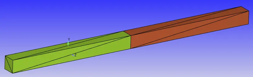
• Inlet & Outlet Boundary conditions: Unlike most simulations which have inlet and outlet boundaries, this simulation is peculiar since we are only going to be using initialized values and wall boundary to isolate the system from surroundings and simulate the internals.
• Wall: All the walls have been given a law-of-the-wall condition, Turbulent Kinetic energy and Dissipation are both marked as zero normal gradient neumann boundaries with temperature boundary of law-of-the-wall condition since we are not resolving viscous sublayer but are modelling it.
• Timestepping and Cycles: Simulation was run for 25000 cycles and in some cases upto 50000 cycles with time minimum time step of 1E-09 and max of 1 second. The convection, diffusion and mach CFLs were kept at standard values of 1, 2 and 50 respectively. The solution was continously monitored and CFL values were appropriately changed to accelerate the convergence rate.
• Event: The HP and LP regions will remain closed till 0.001, after that they will be opened and connected simulating the diaphragm rupture.
• Turbulence Modelling: RANS based K-Epsilon was used with O'Rourke & Amsden wall treatments for heat transfer explained below with different turbulent wall functions depending on situations.

QUICK Reminder from my Conjugate Heat Transfer simulation report (more details : HERE)

Law of the wall boundary conditions means for the simulations with a k-ε turbulence model CONVERGE uses the Launder and Spalding [Launder and Spalding, 1974] wall model for computing (read:modelling) velocity at the wall. This is given by following equation:

For same law-of-the-wall boundary for temperature, O'Rourke & Amsden wall treatments for heat transfer were selected. This is modelled as:

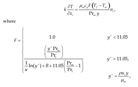
REGION INITIALIZATION:

The high pressure region was initialized with value of 600000Pa and low pressure region with 101325Pa. Major difference was that high pressure region was initialized with 100% N2 in it and low pressure region was initialized with 100% O2.

Turbulence Kinetic Energy was initialized at 1`m^2/s^2` and Turbulent dissipation with 100 `m^2/s^3`

What is Sod's shock tube experiment ? And why is that so important?

The Sod shock tube problem, named after Gary A. Sod, is very common experiment run to validate various phenomena like shocks and information propagation in hyperbolic systems and hence test for the accuracy of CFD codes and was investigated by Sod in 1978. This specific experiment is used widely used for validation because it isolates shocks in system effectively preventing other disturbances from creeping in and hence making job easier for engineer. Another reason why this is widely used is because of the availibility of validation data as it has been performed several times.

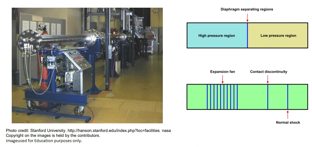
The setup has something similiar to what we have tried to simulate. On one side there is a high pressure state and on the other side there is a low pressure state with a diaphragm separating them from each other. The picture shows how the setup is long and has various probes and gauges to make measurement, usually there is a mechanism to develop high pressure with a compressor on HP side and to rupture the diaphram. On the LP side there are various highly sensitive transient pressure sensors, they are used to track and trace the moving normal shock wave formed in the domain. Eventually those traced movements can be used to calculate the Mach number of wave and validate CFD codes. This ensures the code gives physical solutions to supersonic flows having hyperbolic nature of PDEs.

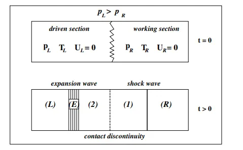
At time t = 0.001 the diaphragm breaks, effectively connecting the two regions where they will try to equalize in pressure. The N2 at the HP expands through an expansion (or rarefaction) wave and flows left into its region. The rarefaction is a continuous process and takes place inside a well-defined region (the expansion fan) that propagates to the left (labelled-E); the expansion fan also gets wider with time. Meanwhile, just opposite to the expansion wave there is a normal shock wave which goes on into right side LP domain compressing it. The expanded gas on left (due to expansion fan) and the compressed gas on the right ( due to shock wave) are still separated at the contact discontinuity which is initially at the diaphragm's postion and moves to the right as time progresses.

It should be noted that the conservative variables defining the flow in the tube (p(x), ρ(x), T(x), and U(x)) are discontinuous across the shock wave and the contact discontinuity. These discontinuities are what cause difficulty in accurate modelling of this experiment as this requires an approximation of Riemann problem at such cell interfaces and hence the values have to be propagated based on the 'characteristic values' (read: eigen value of formulated matrix) of the system.

EXACT SOLUTION:

Below is just a brief of calculation for exact solution of Eulerian equations (inviscid) for above mentioned shocktube problem. Considering this problem in 1D and (x,t) space as shown below we can easily calculate the 1D solutions.

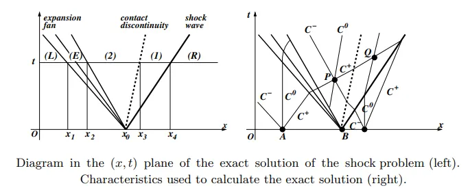
As we can see for shock between (1) and (R) regions we can apply Rankine Hugoniot's jump relation across shockwave. Notice the shockwave would mean there is a discontinuity across all the conservative variables in domain.

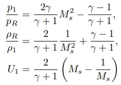
where Ms is the mach number of shock.

On the other hand, with only a contact discontuinty between (1) and (2), so only density is discontinuous at such position. (which should also be validated in CFD code)

Information propagating in system can be better understood by considering 'method of characteristics' for solution matrix. The underlying idea is here to generalize the analysis of characteristics in the case of a system of PDEs especially hyperbolic PDEs in case of super sonic flows. Some conservation variables are classified as invariants, they are transported along particular curves in the plane (x, t) called characteristics. This characteristics are plotted on the figure above as seen on the right, now consider point P inside the region (2) and draw the characteristics passing through this point. We notice that only C0 and C+ characteristics will cross the expansion fan to search the information in region (L). Using the 'method of characteristics' we can determine invariants on the characteristic curve and get following relations.

and then we can go on to calculate

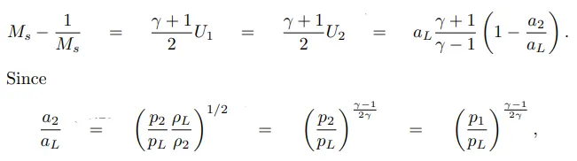
we get final equation which is formulated implicitly and has to be solved iteratively. Once Ms is computed, rest of all the properties above can be calculated.

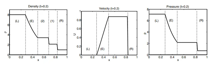
After all this the solution of the equation should look something like this, the exact values might be different but each solution must give such characteristic shape. We should be seeing similiar curve in our solution as well.

What is a shock? And why does it occur anyway?

Shocks are fundamentally a discontinuity or an abrupt change in flow field properties in a domain. Shock flows are most commonly known and encountered around the supersonic aircrafts, almost everyone has seen and heard of a distinct loud sound of an airplane flying over the speed of sound and has also seen a condensation cloud forming around the aircraft also called as vapour cone or shock cone. The cloud formation is because every high pressure shock wave front there is a normal or expansion zone, which is where air cools down and the moisure condenses to form that signature cone shape.

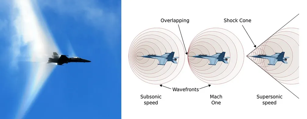
What happens when a body is moving faster than the speed of sound itself in the domain, the information which is communicated through domain at speed of sound is actually not fast enough. This causes the sound waves or disturbances in the medium to 'pile up' and at the region where the waves 'add up' there is a huge pressure discontinuity which moves into the domain as a shock wave

More on this in my other article : HERE

In this simulation we will be dealing with Normal shock wave propagating in the medium.

3. RESULTS

Here we have ploted various contour plots and line plot along the domain to validate our code and check our simulation. It would be much better to watch videos more than pictures and plots as they will provide much better insight on what actually is happening.

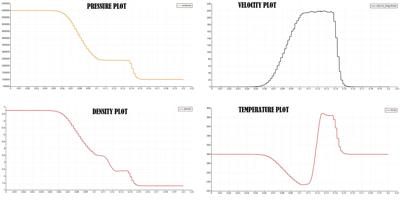
For initial results, we can see their shape after time t= co-relates well with our previous exact solution image. We can see the shock propagating in the right LP domain and a rarefaction wave propagating in the HP domain with a density discontinuity in the middle moving right. This is exactly what we were looking for in our solution and validates well with our expectations and exact solution.

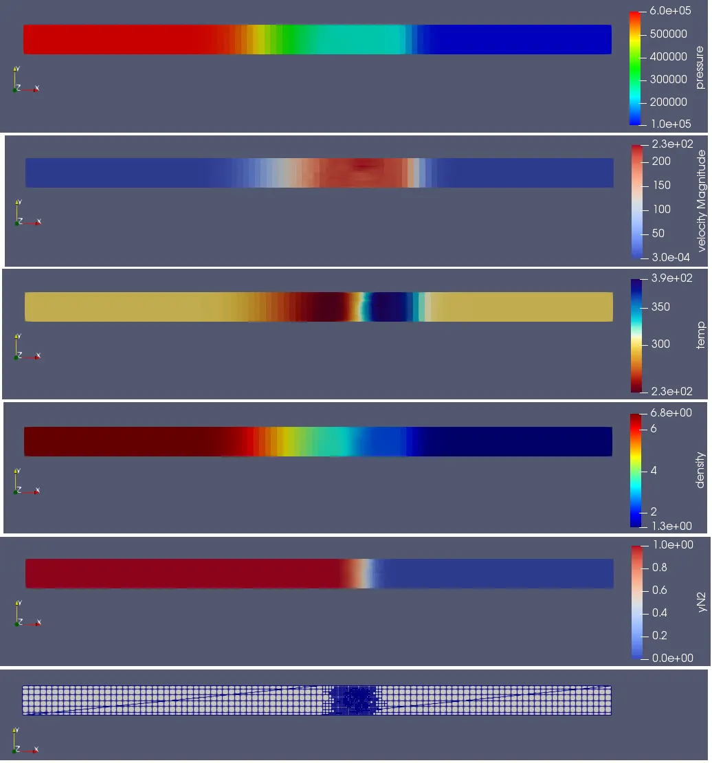
Besides looking at the snapshot of contour, it would make much more sense to look at the dynamic plots side by side as below. With this you will have much better idea, one can also see the shocks being reflected. The mechanism here to think about is shock is a type of pressure discontinuity advancing as a front, when this high pressure wave hits the wall it bounces back and travels the other way. But as it propagates through the medium its intensity decreases as its energy slowly dissipates.

Adaptive Mesh Refinement:

As we have already seen above, Converge requires minimal input from the user's end for its own mesh generation. It automatically generates the best possible cartesian mesh for its domain. Ideally we would want as coarse mesh as possible with refinements at the places only and only where it is absolutely needed. The AMR algortihm of converge does just that, it adds embedding determined by algorithm to the portion of domain where the flow field variables are least resolved or so to speak where sub-grid field is largest. In simple words, it will check for the curvature gradients of the variable in the spatial domain and compares it to user defined tolerance.

In converge, this subgrid field is defined as a difference of actual field and resolved field,

The sub-grid for any scalar can be expressed as an infinite series (Bedford and Yeo
(1993) and Pomraning (2000), as is given by

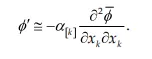
Since it is not possible to evaluate the entire series, only the first term (the second-order
term) in the series is used to approximate the scale of the sub-grid :

A cell is embedded if the absolute value of the sub-grid field is above a user-specified value.
Conversely, a cell is released (i.e., the embedding is removed) if the absolute value of the
sub-grid is below 1/5th of the user-specified value.

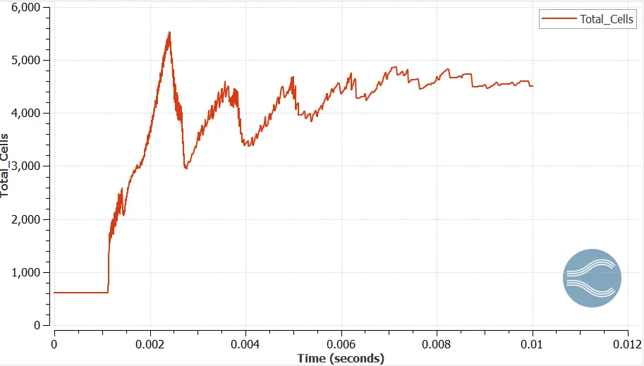
For this particular simulation we used species based embedding with SGS parameter of 0.001 and maximum cells of 200000. SInce our simulation was only 2D, we didnt have to worry about maxing out our cell count. This also means that we will be seeing more refined solution when it comes to species concentration. The cell count is continuously changing as the species intermix and shock wave passes over it further energizing it.

Back to Shocktube Simulation:

Some convergence plots which were monitored to check if the simulation was converging or not are shown below:

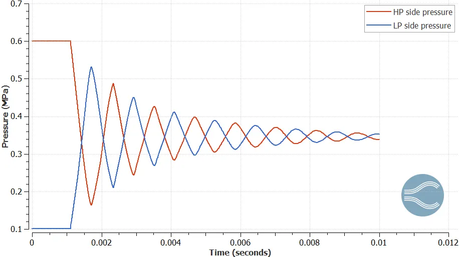
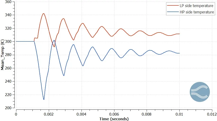
Some more contours of conservative properties played side by side with their plot, this show exactly how the shock propagates and all the 5 regions are clearly seen before first shock reflection at the end of LP domain. This will clarify all the minor doubts highlighting the changes side by side.