Transient Structural Analysis on the Long Piston and Cam Model 

Transient Structural Analysis on the Long Piston and Cam Model

Aim :

• To perform Transient Structural Analysis on the Long Piston and Cam Model with three different materials.

Objective :

• To define appropriate materials to the Piston and Cam Model.
• To define connections between them.
• To perform mesh on the Cam and Piston Model.
• To define appropriate Boundary Conditions to the Model.
• To solve and compare the results of the three cases for Total Deformation, Von-Mises Stress, and Equivalent Elastic Strain.

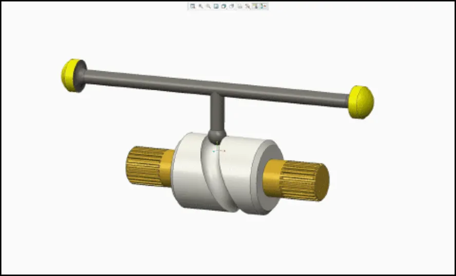
Figure 1-Long Piston and Cam Animation.

Procedure :

Phase 1- Material Set-Up :

• To set up the material for the Rolling Operation Model. First, drag and drop the transient structural analysis workspace into the project schematic from the analysis system. This is shown in below Figure 2.

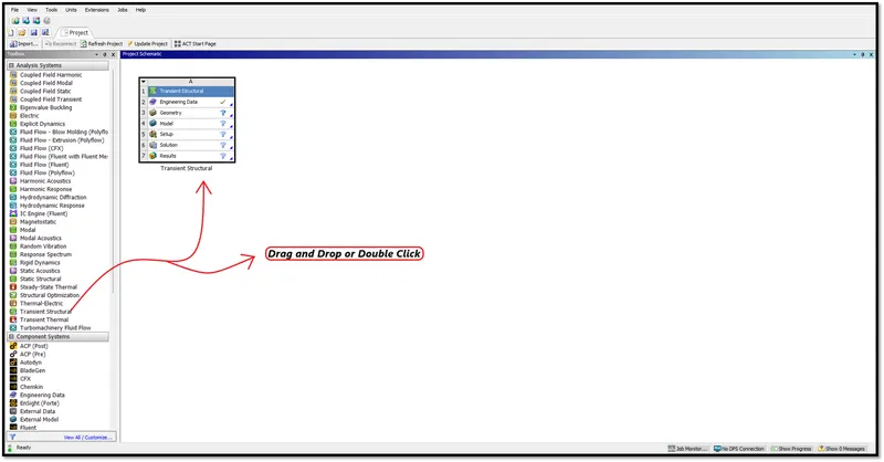
Figure 2-Ansys Workbench Workspace.

• After deploying the transient structural analysis system in the project schematic workspace.
• Define the Engineering Data and geometry, To define the Geometry and Engineering Data, Right Click on the Engineering Data and click to edit, it will take to the Engineering Tab.
• There Right Click on the Material Tab, A window will Pop-Up stating Engineering data sources.
• Click on the Engineering Data Sources, There go and select the material to define the engineering data. This is shown in below Figures 3,4,5.

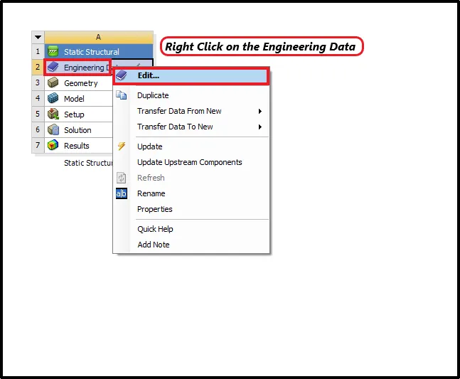
Figure 3-Right Click on the Engineering Data.

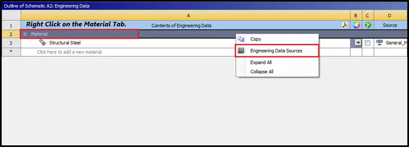
Figure 4-Right Click on the Material Tab.

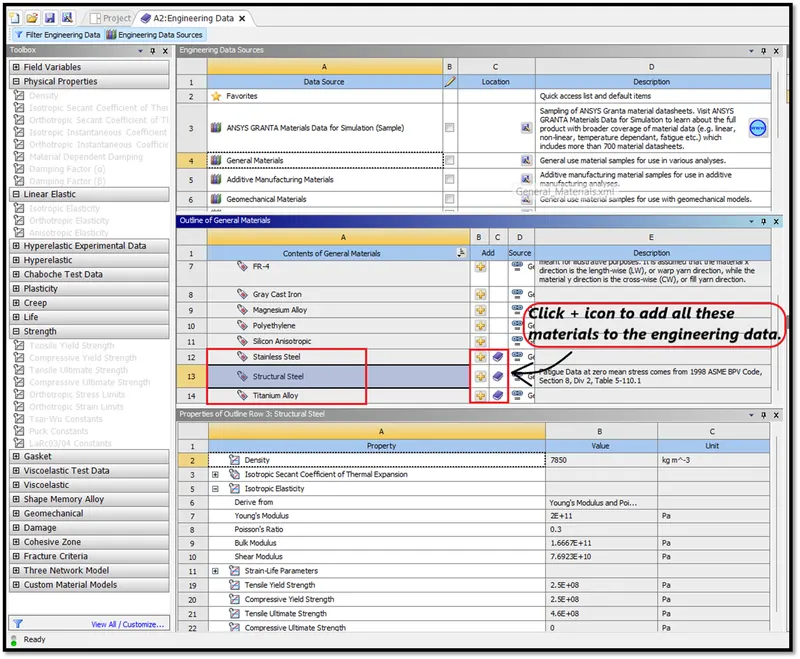
Figure 5-Select these Materials to define the Model.

Phase 2-Geometry Set-Up :

• Next set up the geometry. To set up the geometry, Right-Click on the Geometry option >> Import Geometry. This is shown in below Figure 6.'

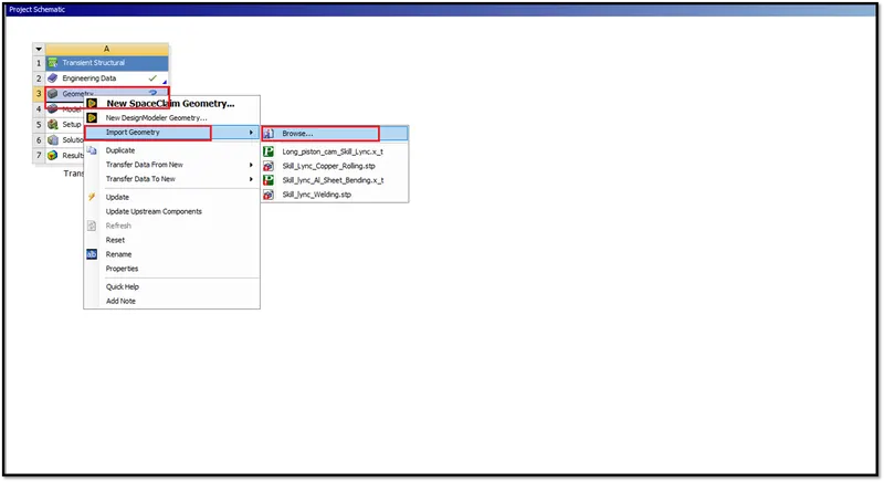
Figure 6-Importing Geometry.

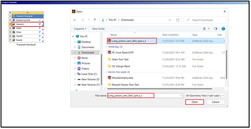
Figure 7-Selecting the Geometry to Import.

• Next double click on the geometry to check, Whether the model imported, is Long Piston and Cam Model or not. Space Claim Workspace will open. The model will be imported in the space claim, Which is shown in below Figure 8.

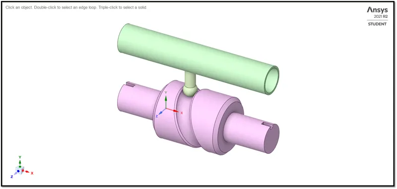
Figure 8-Long Piston and Cam Model in the Space Claim.

Phase 3-Model Set-Up :

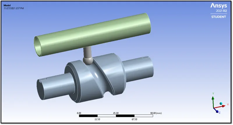
• Next, define the model, Double click on the model, The Mechanical Workspace will open, There go and define the material, set up the load case for the model.
• The Model loaded in the mechanical workspace is shown in below Figure 9.

Figure 9-Model Loaded in Mechanical Workspace.

3:1 Assign Material :

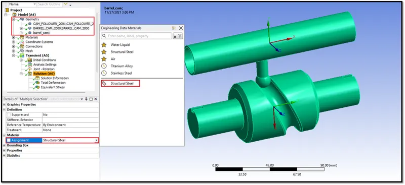
• Next, define the material as Structural Steel for the Long Piston and Cam Model which is shown in below Figure 10.
• To assign a material,Click on the Geometry >> Select the Long Piston and Cam Geometry >> Parameter Window >> Assignment >>Structural Steel.
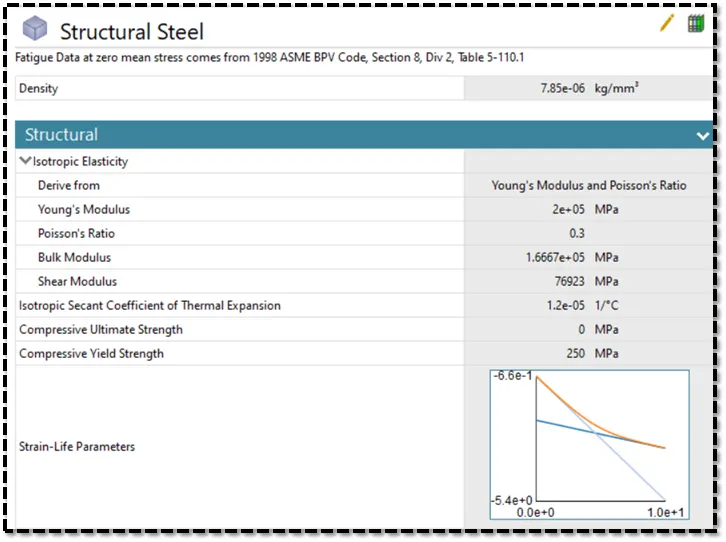
• The mechanical properties of the material are shown in below Figure 11.

Figure 10-Assign Material to the Long Piston and Cam Model.

Figure 11-Mechanical Properties of Structural Steel.

3:2 Define Connections :

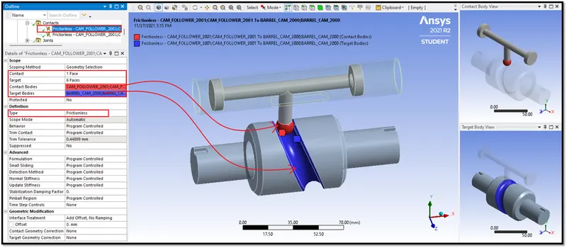
• For this Long Piston and Cam Model, We have to Create two contacts, One is between Cam Follower and Barrel and the other one is between Cam Follower and Barrel Cam.

1) Contact between Cam Follower and Barrel Cam:

• Select the cam follower as a Contact Body and Select the groove faces as a Target Body,Which is shown in Figure 12.
• Case 1, Type of Contact is "Frictionless", There will be no frictional force or resistive force between that component.
• Case 2, Type of Contact is "Frictional" with Frictional Coefficient is 0.1.
• Case 3, Type of Contact is "Frictional" with Frictional Coefficient is 0.2.

Figure 12-Defined Contact between Cam Follower and Barrel Cam.

2) Contact between Cam Follower and Barrel :

• Select the piston face as the Contact Body and select the barrel face as the Target Body, Which is shown in below Figure 13.

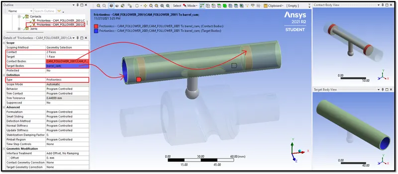
Figure 13-Defined Contact between Cam Follower and Barrel.

3:3 Define Joints :

• We have to define three joints to this Long Piston and Cam Model.

1) Fixed Joint :

• Select the barrel outer face to give fixed joint, where all the degrees of freedom will be constrained,Which is shown in below Figure 14.

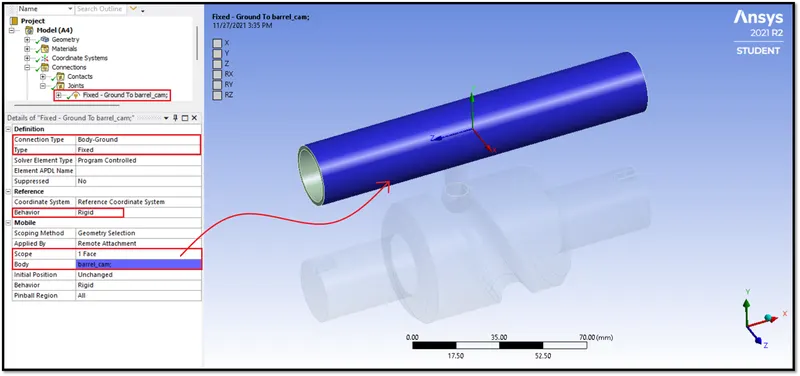
Figure 14-Defined Fixed Joint.

2) Revolute Joint :

• To define the revolute joint, We have to select the face which is shown in below Figure 15.

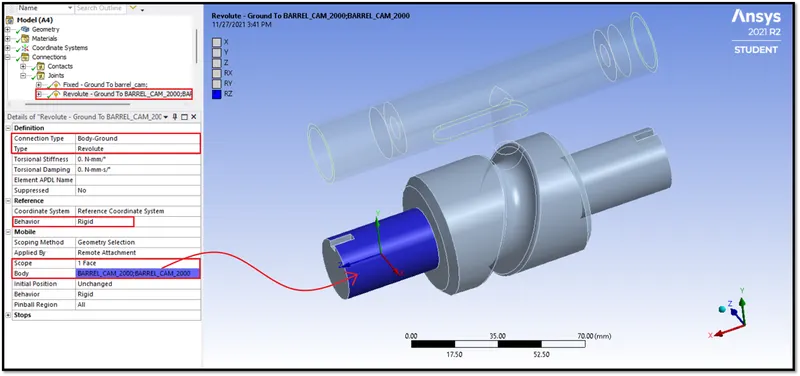
Figure 15-Defined Revolute Joint.

3) Translational Joint :

• We have to select the outer face of the barrel and the inner face of the piston, Cause barrel should translate along the X-axis, Which is shown in below Figure 16.

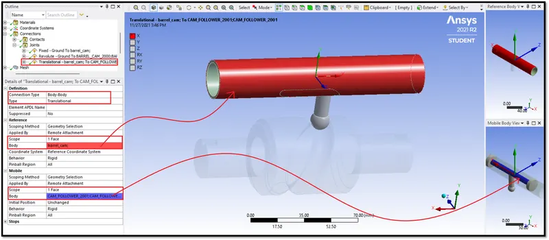
Figure 16-Defined Translational Joint.

3:4 Meshing :

• After defining the connections, We have to define mesh for the Long Piston and Cam Model.

• To get the results accurately between the cam follower and Barrel cam. We have to refine the mesh by using Face sizing with an element size of 3 mm. In this way, we can capture accurate results.

• Note: Go to the Mesh Details and Change Adaptive Sizing to No.

• To Insert Face Sizing >> Right Click on Mesh >> Insert >> Sizing >> Select Barrel Cam Faces and Cam Follower.This is shown in below Figure 18.

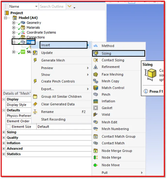
Figure 17-Insert Face Sizing to Refine the Mesh.

1) Face Sizing :

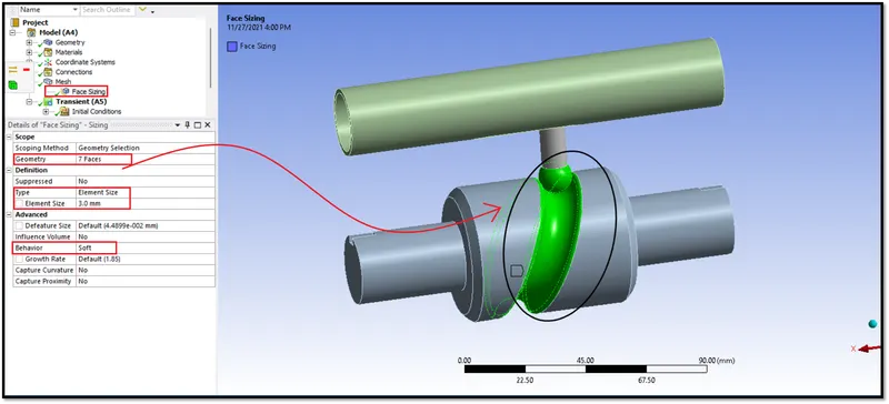
Figure 18-Face Sizing.

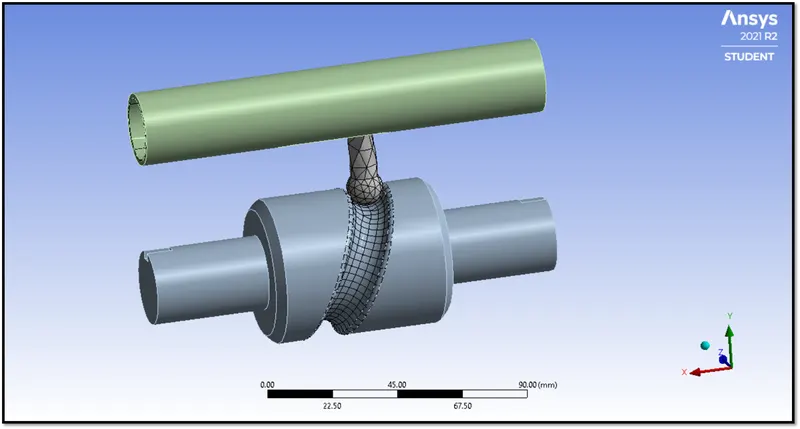
Figure 19-Final Meshed Model.

• Here we have changed the behavior to rigid for Barrel and Barrel cam. So the meshing has not been done for the whole component,
• We had made surface mesh with mixed types of elements.

3:5 Analysis Settings :

• Here for this Long Piston and Cam Model, We are giving 9 steps to run the simulation.

Step-1 :

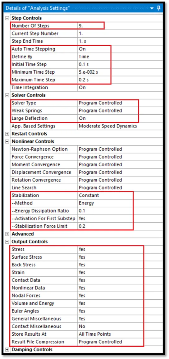
Figure 20-Analysis Setting for Step-1.

Step 2-9 :

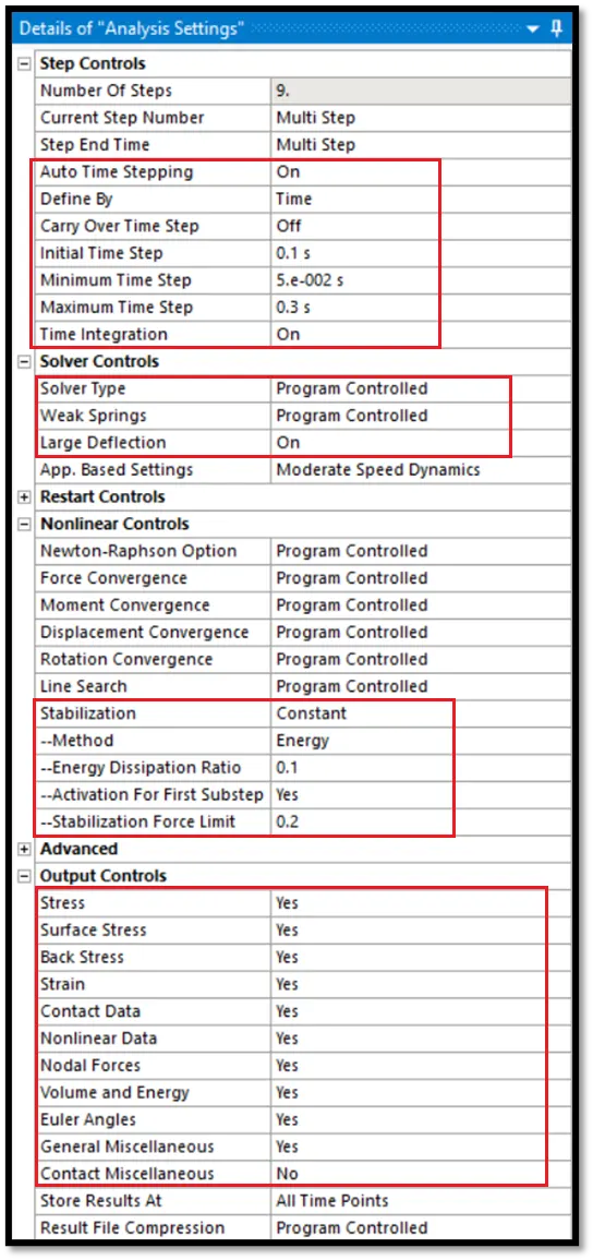
Figure 21-Analysis Setting for Step 2-9.

3:6 Boundary Conditions :

• After giving some parameters in the analysis settings, We have to give boundary conditions.
• Here we have to create only one boundary condition, Joint Rotation.
• To give Joint Rotation, Right Click on the Static Structural >> Insert >> Joint Rotation. This is shown in below Figure 22.

1) Joint Rotation :

• Select the Ground to Barrel Cam for the type of joint.
• Select Rotational for the type of definition.
• The barrel cam should rotate from 0 degrees to 270 degrees with an equal interval of 9 steps.

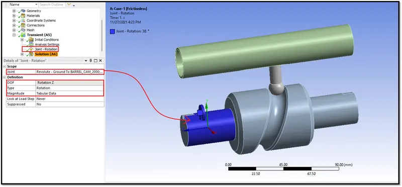
Figure 23-Defined Rotational Joint.

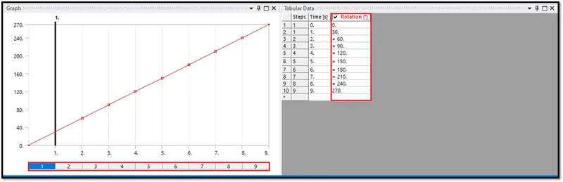
Figure 24-Values given in the Tabular Data for Rotation.

Phase 4-Request for the Outputs :

• Here we have to request outputs for the VonMisses Stress, Strain, and for Total Deformation.
• To request Output for Stress,Right Click on the Solution >> Insert >> Stress >> Equivalent Von Misses Stress.
• To request Output for Strain,Right Click on the Solution >> Insert >> Strain >> Equivalent Von Misses Strain.
• To request Output for Total Deformation,Right Click on the Solution >> Insert >> Deformation >> Total Deformation.
• This is shown in below Figure 25.

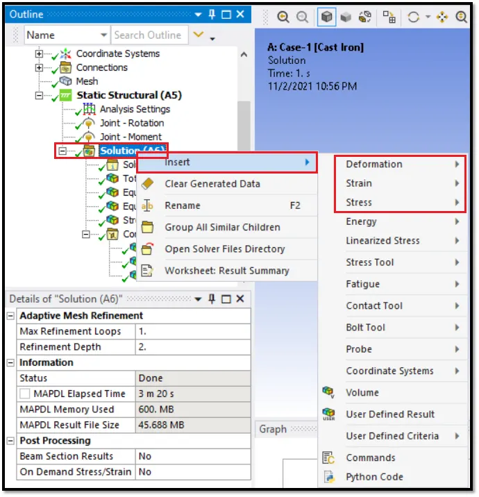
Figure 25-Requesting Outputs for the Stress, Strain, and Deformation.

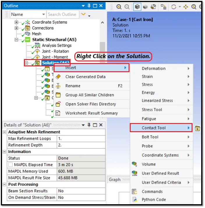
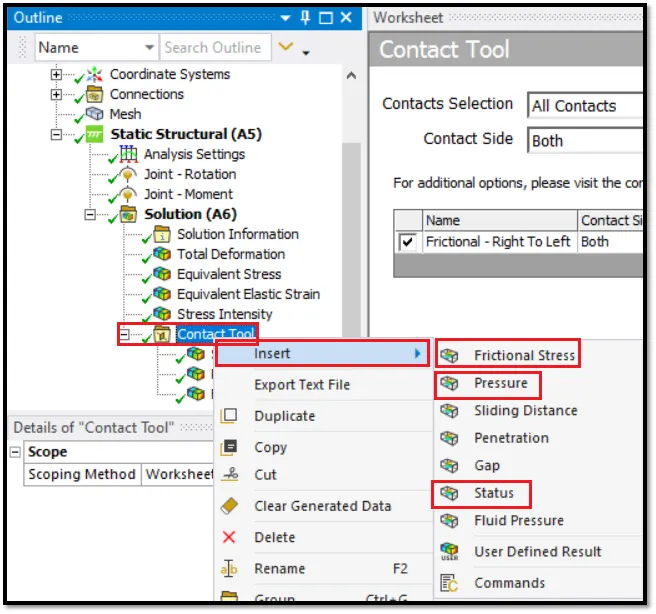
• Next request output for the contact.
• To request Contact Tool >> Right Click on the Solution >> Insert >> Contact Tool >> Pressure >> Status,Which is shown in below Figures 26 and 27.

Figure 26-Requesting Output for Contact.

Figure 27-Requesting Outputs for Contact Tool.

• Similarly request the output for the Force Reaction.
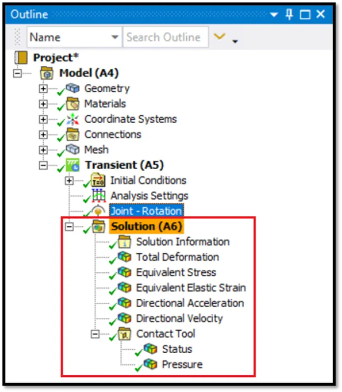
• The Output requested for the Wire Bending Model is shown in Figure 28.
• After requesting all the outputs, Run the Simulation.

Figure 29-Required Outputs Requested.

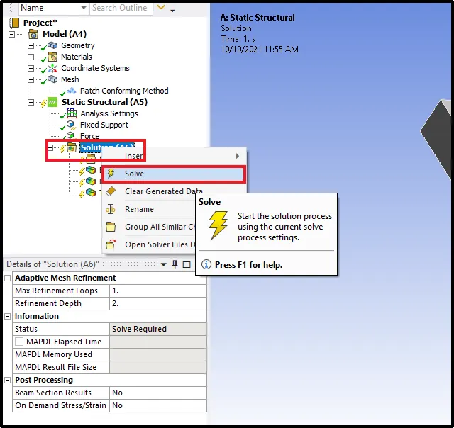
• To run the simulation, Right Click on the Solution >> Solve. This is shown in below Figure 30.

Figure 30-Solve all the Outputs Requested.

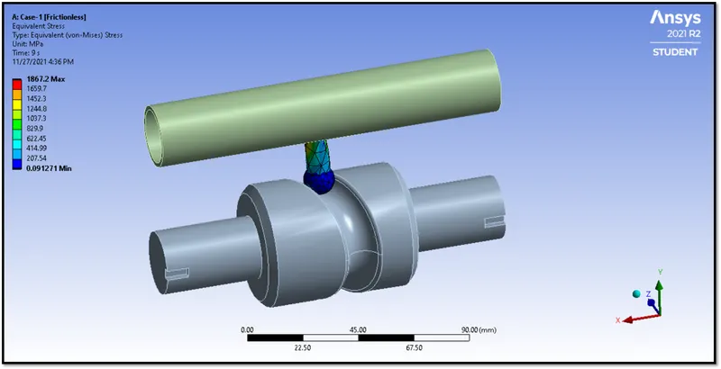
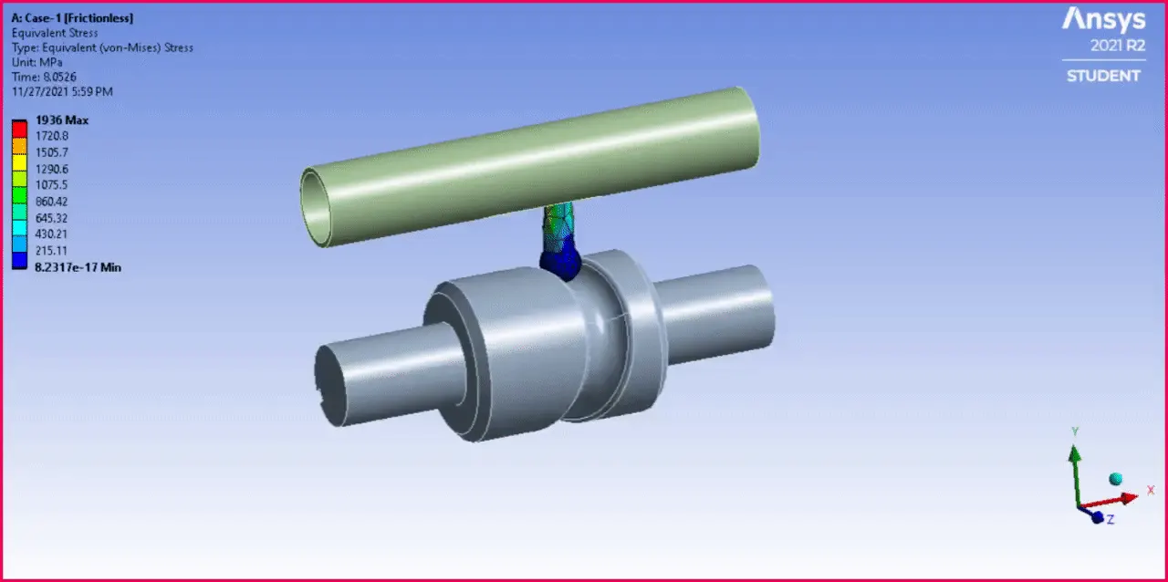
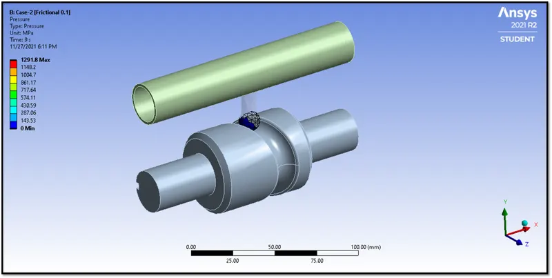
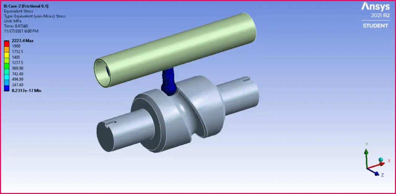
• After solving the outputs requested, the simulation results for all three cases are shown below Figures.

Case 1 [Equivalent Von Misses Stress Frictionless] :

Figure 31-Equivalent Von Misses Stress [Case 1-Frictionless].

Figure 32-Equivalent Von Misses Stress Simulation Animation [Case 1-Frictionless].

Case 2 [Equivalent Von Misses Stress Frictional with Coefficient of 0.1] :

Figure 33-Equivalent Von Misses Stress [Case 2-Frictional Coefficient of 0.1].

Figure 34-Equivalent Von Misses Stress Simulation Animation [Case 2-Frictional Coefficient of 0.1].

Case 3 [Equivalent Von Misses Stress Frictional with Coefficient of 0.2] :

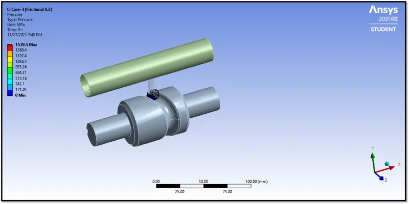
Figure 35-Equivalent Von Misses Stress [Case 3-Frictional Coefficient of 0.2].

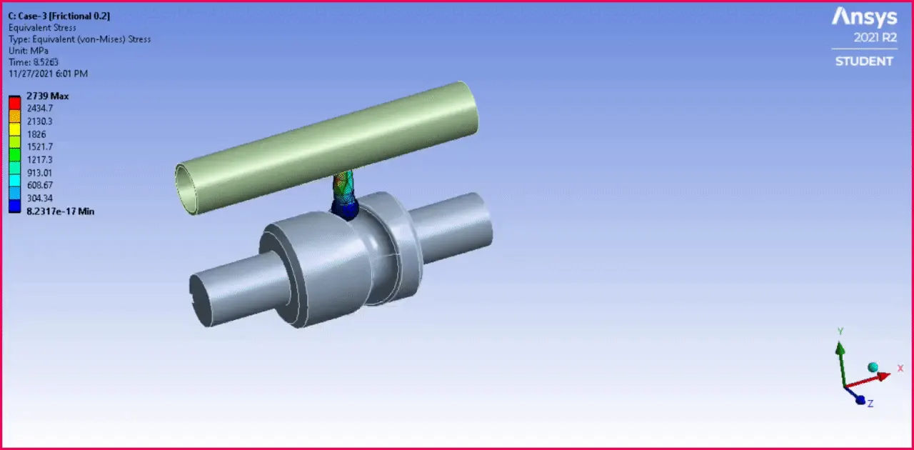
Figure 36-Equivalent Von Misses Stress Simulation Animation [Case 3-Frictional Coefficient of 0.2].

Case 1 [Equivalent Elastic Strain Frictionless] :

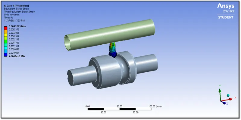
Figure 37-Equivalent Elastic Strain [Case 1-Frictionless].

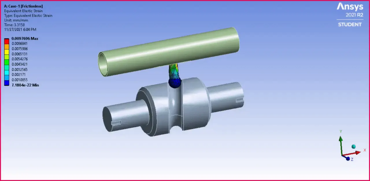
Figure 38-Equivalent Elastic Strain Simulation Animation [Case 1-Frictionless].

Case 2 [Equivalent Elastic Strain with Frictional Coefficient of 0.1] :

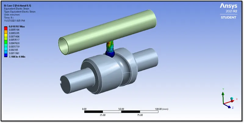
Figure 39-Equivalent Elastic Strain [Case 2-Frictional Coefficient of 0.1].

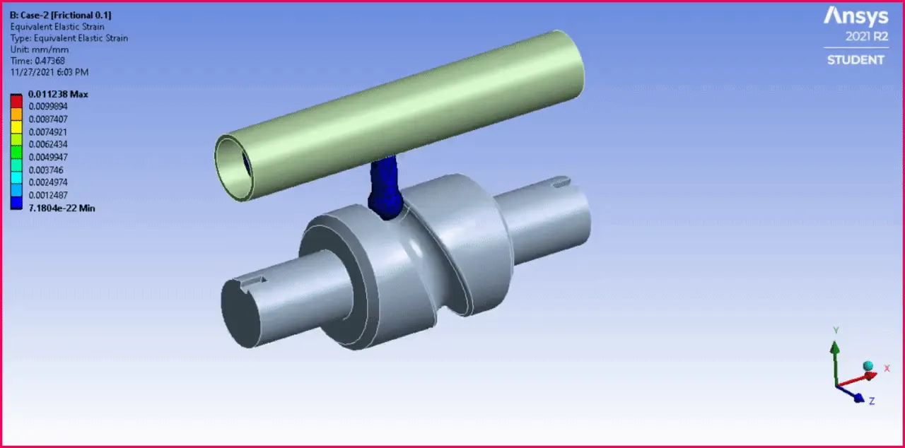
Figure 40-Equivalent Elastic Strain Simulation Animation [Case 2-Frictional Coefficient of 0.1].

Case 3 [Equivalent Elastic Strain with Frictional Coefficient of 0.2] :

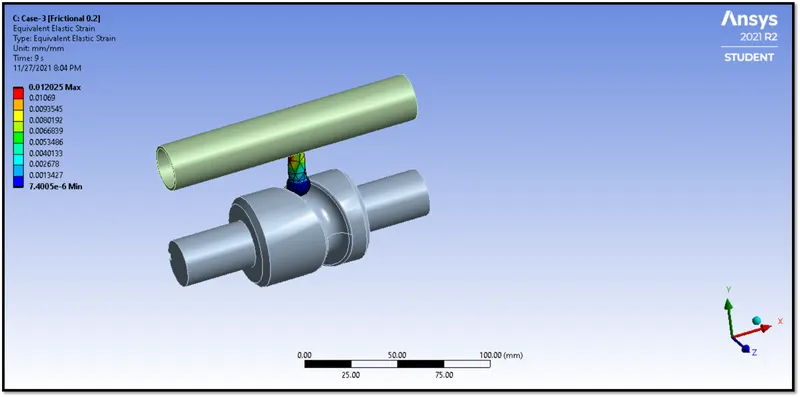
Figure 41-Equivalent Elastic Strain [Case 3-Frictional Coefficient of 0.2].

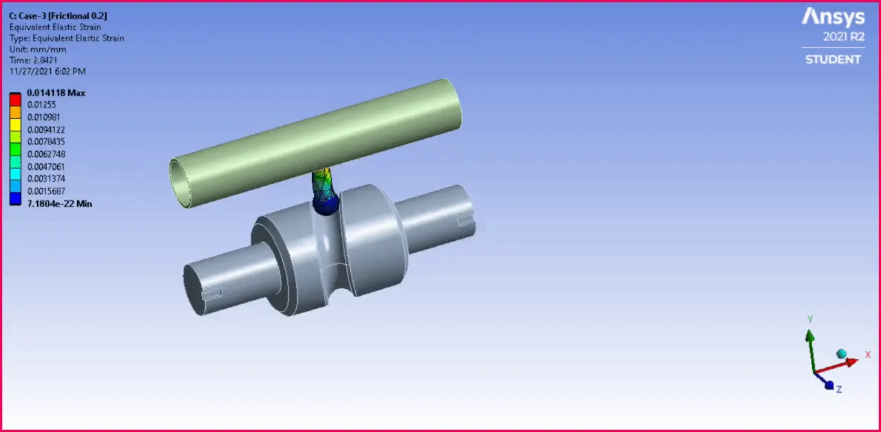
Figure 42-Equivalent Elastic Strain Simulation Animation [Case 3-Frictional Coefficient of 0.2].

Case 1 Total Deformation :

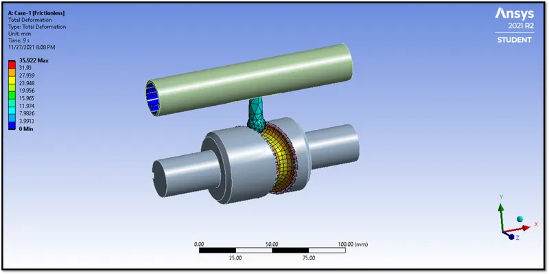
Figure 43-Case 1 Total Deformation.

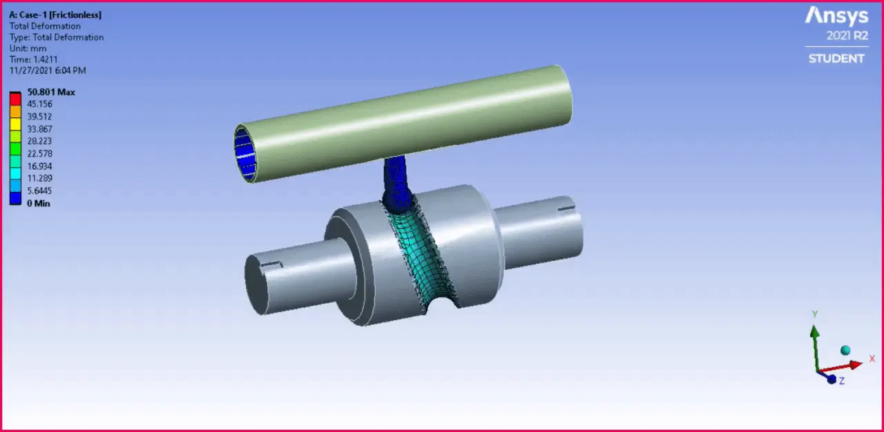
Figure 44-Case 1 Total Deformation Simulation Animation.

Case 2 Total Deformation :

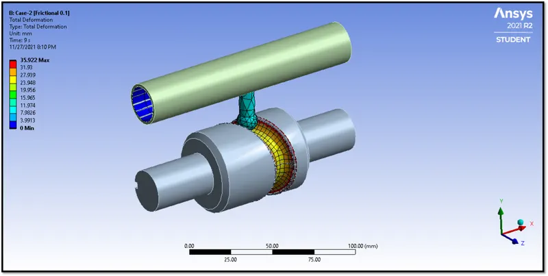
Figure 45-Case 2 Total Deformation.

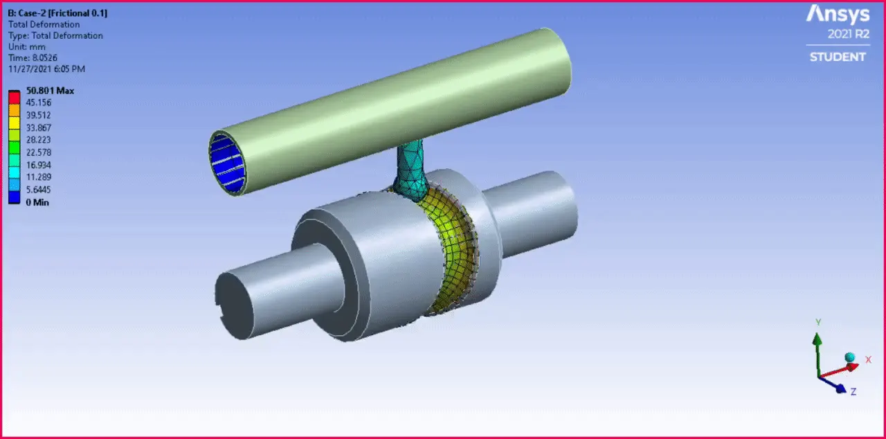
Figure 46-Case 2 Total Deformation Simulation Animation.

Case 3 Total Deformation :

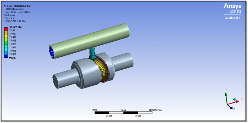
Figure 47-Case 3 Total Deformation.

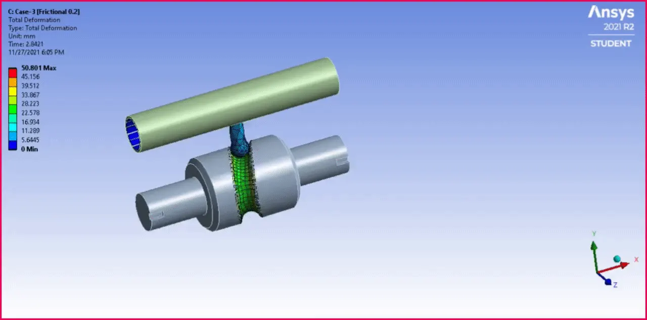
Figure 48-Case 3 Total Deformation Simulation Animation.

Case-1 Directional Acceleration :

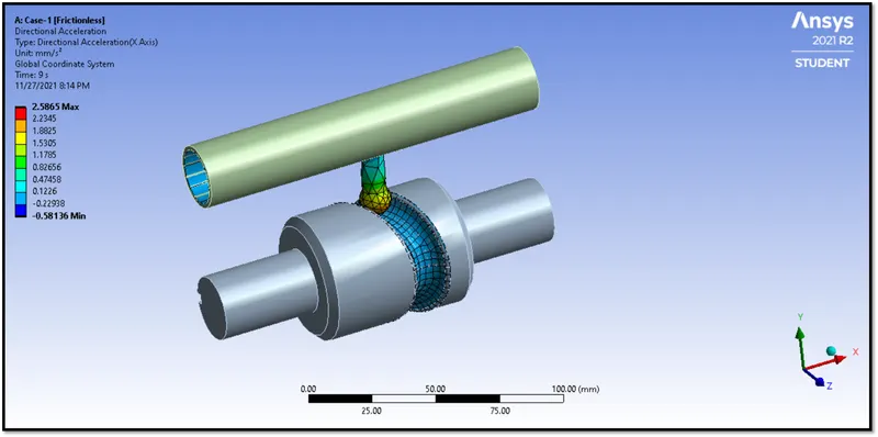
Figure 49-Case 1 Directional Acceleration.

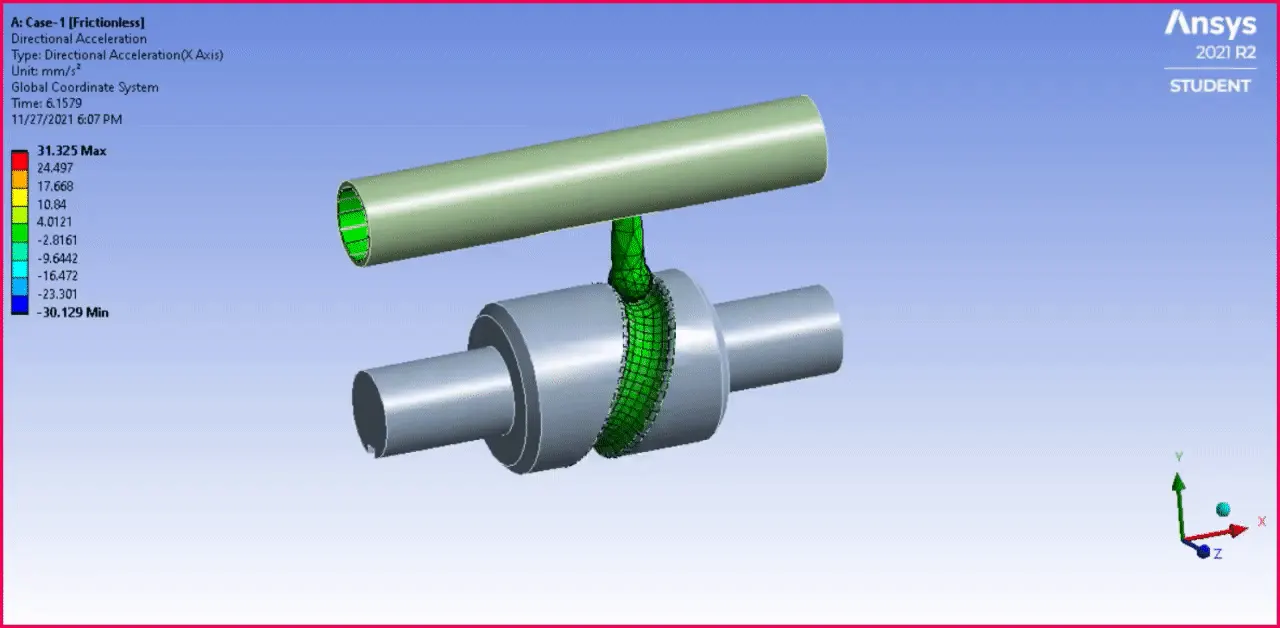
Figure 50-Case 1 Directional Acceleration Simulation Animation.

Case-2 Directional Acceleration :

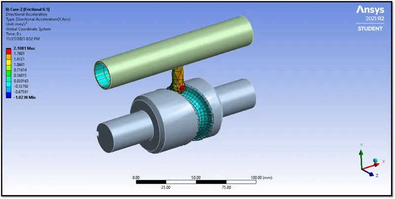
Figure 51-Case 2 Directional Acceleration.

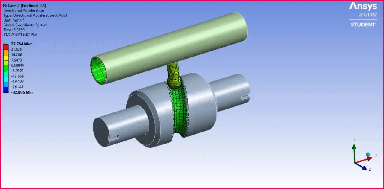
Figure 52-Case 2 Directional Acceleration Simulation Animation.

Case-3 Directional Acceleration :

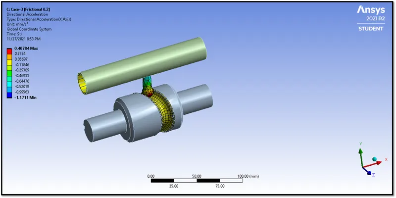
Figure 53-Case 3 Directional Acceleration.

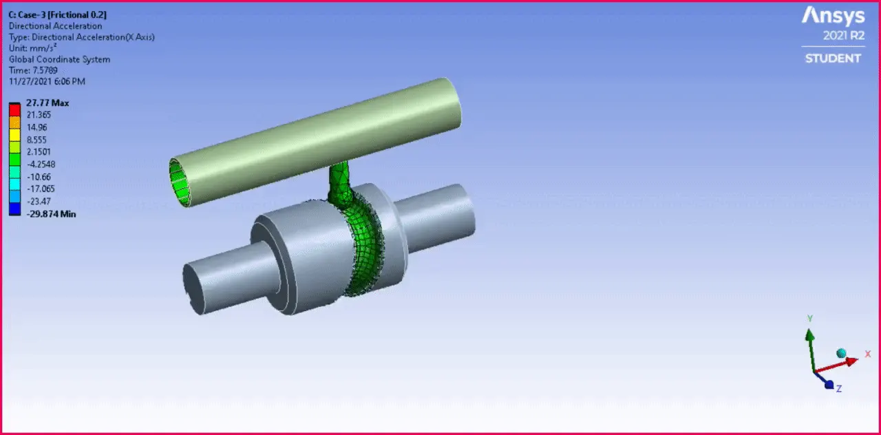
Figure 54-Case 3 Directional Acceleration Simulation Animation.

Case-1 Directional Velocity :

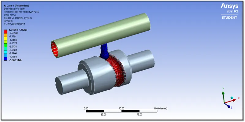
Figure 55-Case 1 Directional Velocity.

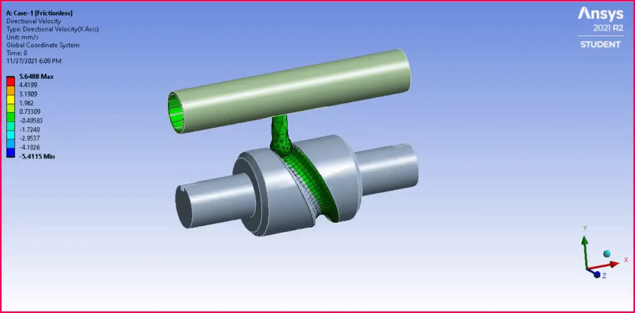
Figure 56-Case 1 Directional Velocity Simulation Animation.

Case-2 Directional Velocity :

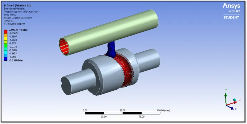
Figure 57-Case 2 Directional Velocity.

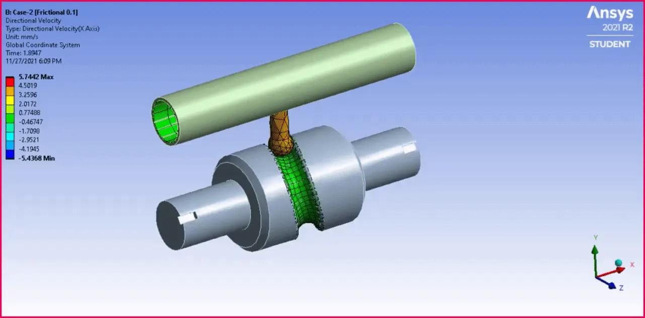
Figure 58-Case 2 Directional Velocity Simulation Animation.

Case-3 Directional Velocity :

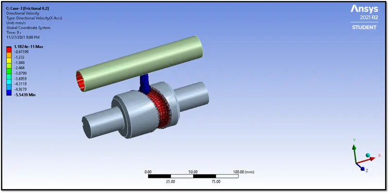
Figure 59-Case 3 Directional Velocity.

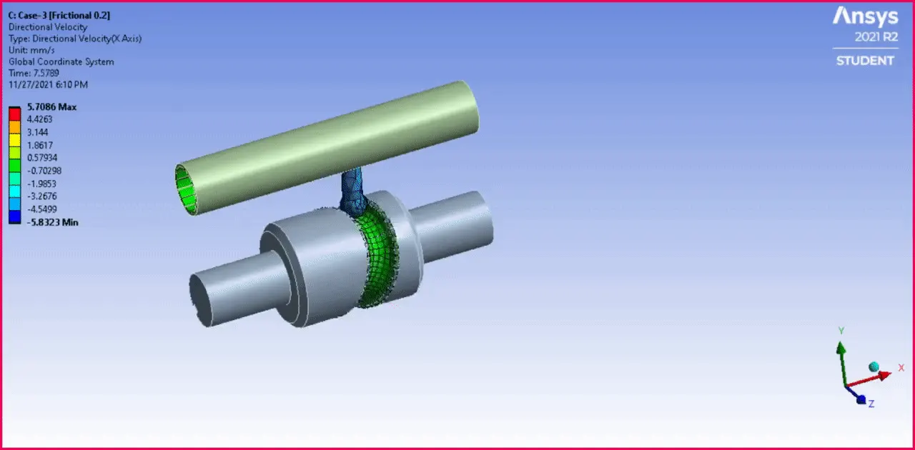
Figure 60-Case 3 Directional Velocity Simulation Animation.

Results :

Cases	Equivalent Von-Misses Stress (MPa)		Equivalent Elastic Strain (mm/mm )		Total Deformation (mm)
	Max.	Min.	Max.	Min.	Max.	Min.
Case-1 Frictionless	1867.2 MPa	9.1271e-002 MPa	9.3793e-003 mm/mm	7.0666e-006 mm/mm	35.922 mm	0
Case-2 Frictional Coefficient of 0.1	2130.5 MPa	9.2973e-002 MPa	1.0707e-002 mm/mm	7.1883e-006 mm/mm	35.922 mm	0
Case-3 Frictional Coefficient of 0.2	2391.2 MPa	9.5764e-002 MPa	1.2025e-002 mm/mm	7.4005e-006 mm/mm	35.922 mm	0

Table-1

• Here from the above results. We came to know, When the coefficient of friction is increased, the value of Maximum Deformation, Von-Misses Stress, and Equivalent Elastic Strain is also increased, because as the coefficient of friction is increased, So the frictional resistance to motion is also increased.
• So the Case-3 with a frictional coefficient of 0.2 has the highest value of stress, strain, and deformation when compared to the other two cases.