Week-7 : Converting a detailed engine model to a FRM model

Understanding and creating a Fast running model in GT-Suite

Aim:

To build a Fast-Running Model in GT-Power

Introduction:

Fast Running Models are dynamic, fully-physical engine models that are designed specifically to run fast. While high-fidelity engine models are commonplace in the engine performance department, they are often too slow running to incorporate into the system level models where long transient events may be simulated, or where the simulation model must respond faster than real -time, such as for hardware-in-loop (HiL) simulations [1].

FRMs achieve such fast run times by two means:

1. Increasing the simulation time step size
2. Decreasing the number of calculations per time step

These two means are often accomplished at the same time by lumping various flow volumes together which will reduce the total number of sub volumes and also allow for a larger time step size by increasing the effective sub volume length (which is responsible for the time step size). In addition to simplifying and combining flow volumes, there are additional solver options that can reduce the number of calculations per time step and, thus, further decrease the run time without changing the time step size [1].

FRMs execute more rapidly than the typical detailed GT-Power engine model. Therefore, they are ideal for integrating with other vehicle systems where an accurate and predictive engine plant model is desired and there the computational speed is critical. FRMs adapt to changing conditions (e.g. Valve timings, turbo lag, etc) without the need to apply non-physical correction factors. They are particularly useful in studying changes to ambient conditions, or simulating events that are heavily transient in nature. FRMs maintain the predictive capabilities of a detailed engine model while allowing for the fast computational speeds that are expected when performing drive cycle analysis and other transient-focused simulations [2].

Some of the examples include [2]:

• ECU Modelling including HiL where a fast-running and transient-capable engine model is essential for optimizing ECU strategy
• Engine + Drivetrain/Vehicle – where accurate torque pulsations are key for optimizing drivetrain design and strategy.
• Vehicle Thermal Management modelling, where the engine provides the heat to the cooling system, and the cooling system behaviours feeds back into the engine performance predictions (great for simulating off-ambient conditions)

Model Creation:

FRM can be created using two methods:

1. Create a detailed high-fidelity model and then convert it into FRM
2. Create a FRM directly using pre-defined templates

This short case-study will explain both the methods briefly.

FRM Converter:

To use this tool, we need a detailed model. In this case-study, the pre-existing example of 4-cylinder SI engine with GDI Turbo was used [1]. The detailed engine model is shown in the figure below. This section is based on the tutorial 9 available in GT-Suite.

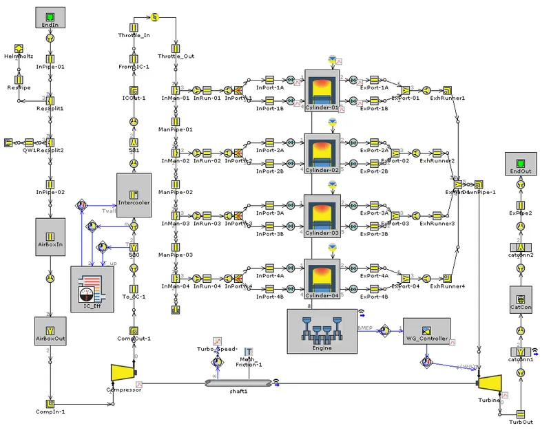
This model is a 4-cylinder 2.0 litre turbocharged Gasoline Direct Injection (GDI) engine. In this model, the turbine wastegate is being dynamically controlled in order to achieve the target BMEP. It also contains a semi-predictive charge air-cooler which predicts the outlet temperature as a function of the inlet gas temperature, mass flow rate, coolant temperature and the air-cooler effectiveness.

To convert the above high-fidelity model into an FRM, the following steps need to be executed.

Step 1: Identify the regions/parts restricting the time-step

In this step, the parts which restrict the overall time-step will be identified. It can be achieved by running the model and plotting the “Minimum Courant Time Step (Explicit Circuit only)” in GT-Post as shown in the figure below. The lower the value, the more likely a part will restrict the timestep. The option “Fraction of timesteps limited by Part” can also be used to identify the parts restricting the timestep.

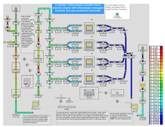
It can be observed from the figure that the following parts restrict the timestep

• Exhaust manifold (parts after the engine and before the turbine)
• Exhaust pipes (parts after the turbine)
• Intake manifold (parts just before the engine indicated in green)
• Intake pipes (parts just after the compressor and before the manifold)
• Flow volumes preceding the compressor

Step 2: Launch FRM tags

In this step, the flow volumes need to be grouped into different categories called tags depending on their relative influence on the overall timestep. In this tutorial, the regions identified in the previous step were created as tags as shown in the figure below

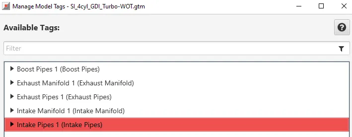
The regions/parts corresponding to the different tags are shown in the appendix.

Step 3: FRM converter

The next step is to open the FRM converter from the base high-fidelity model. Before proceeding further, make sure that the high-fidelity model is run and the respective results are available. The results are required to ensure that the key RLTs are retained accurately within specified tolerances. The FRM converter will compare the key RLTs to keep track of the accuracy of model as the conversion progresses. It will also warn in case a particular RLT becomes outside of a given tolerance.

The following RLTs were specified in this case-study:

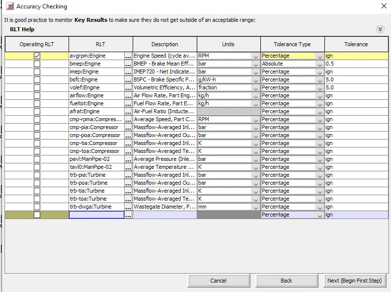
Once the RLTs and their tolerances were defined, the conversion process was started by selecting the “Next (Begin First Step)” option. The conversion process was executed in a series of steps where in each step only a single particular subsystem (FRM tag) was reduced.

Step 4: Start new step

It is most efficient to start by simplifying the part that is currently restricting the timestep. For high fidelity models, this is almost always the exhaust manifold where the highest gas velocities occur, which in turn restricts the time-step. Hence, the Exhaust Manifold 1 tag was selected.

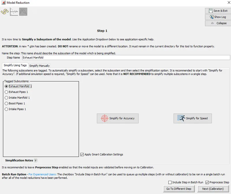
Note: The maximum time step limit of 1 deg should be removed before proceeding further. It will allow for the time step to increase depending on the gas velocity and the sub-volume length.

The model can either be simplified for the accuracy or for speed. In this case, the model was simplified for accuracy. Therefore, the option “Simplify for accuracy was selected.” The exhaust manifold was simplified as shown in the figure below

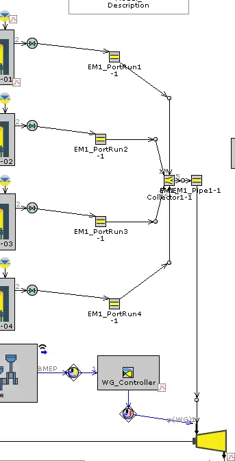
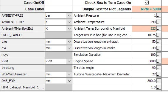
Two parameters were created automatically. One is for the discretization length and the other is for the heat transfer multiplier. These parameters will be optimized to get the required RLTs. The discretization length was set to 300 mm.

Step 5: calibration

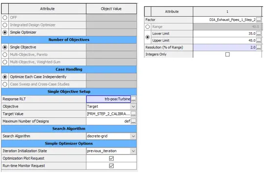
In this step, the case for which the simplified model parameters will be optimized was selected. Here, only the high-speed case (case 1) was selected. Next the calibration was configured. Here the response RLT – the parameter whose accuracy is to be maintained – and the factor parameter – whose value should be changed to achieve the target.

In this case, the response RLT was selected as “mass-averaged turbine inlet temperature” and the “heat transfer multiplier” for the simplified exhaust manifold was selected as the factor.

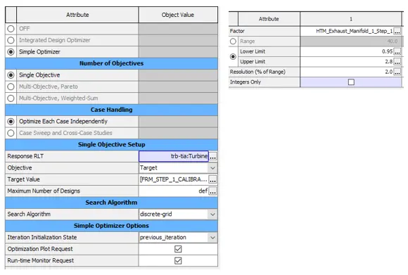
Once the values are selected, the “Run Calibration” button was clicked to start the calibration process. It will optimize the factor parameter to achieve the required target parameter from the baseline model.

Step 6: Run all the cases

In the Results page, the “Run Model” option was selected to run all the cases with the recently tuned parameters. After the simulation was completed, all the key RLTs were compared with the baseline case using the “Populate Accuracy RLT Table Below” option in the results page.

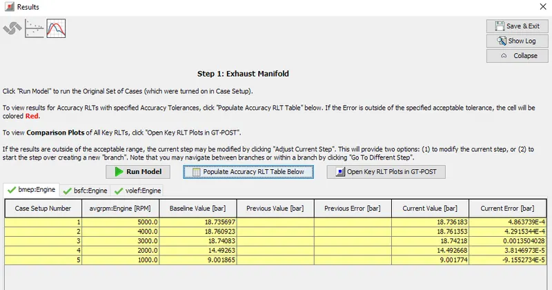
Step 7: Repeat the steps for other sub-volumes

The steps 4,5,6 was repeated for the other sub-volumes defined in step 2. For each sub-volume, care was taken in selecting the right target and factor parameter for optimization.

The parameters used for different sub-volumes are summarized in this table

Sub-volume (FRM tag)	Response (baseline parameter)	Factor (parameter to be modified to achieve the correct response)
Exhaust Pipes	Turbine Mass flow-averaged Outlet Pressure	Exhaust pipe diameter
Intake Manifold	Compressor Mass flow -averaged Outlet Pressure	Intake Heat Transfer Multiplier
Boost Pipes	Compressor Mass flow -averaged Outlet Pressure	Intake pipe diameter
Intake Pipes	Compressor Mass flow -averaged Inlet Pressure	Intake pipe diameter

The progress of the model when the individual subvolumes were simplified are shown below:

Exhaust pipes:

After simplifying for the accuracy

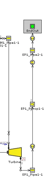
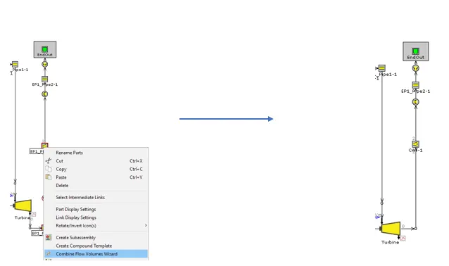
It was observed that the exhaust pipe (with part name ) has limited volume and it still restricts the time step. To overcome this, the exhaust pipe was combined with the catalyst volume into a single flow split manually.

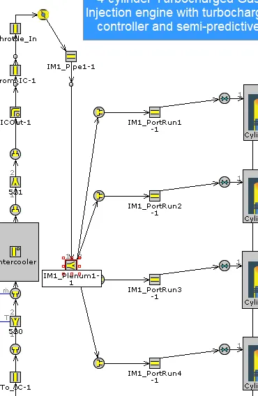
Intake Manifold:

After simplifying for accuracy, the model is reduced as shown in the figure.

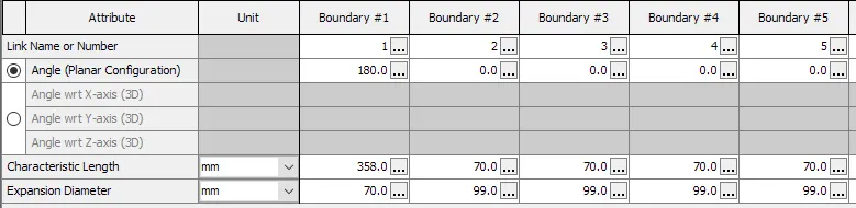
Small modifications were undertaken for the characteristic length and the expansion diameter as shown in the following figure

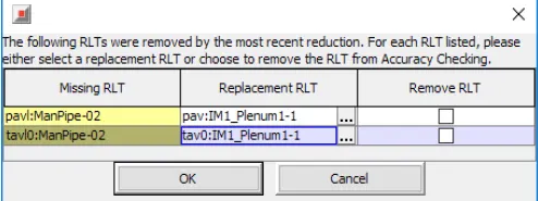
Since the inlet manifold is reduced, the part used to calculate the volumetric efficiency (Manifold) was replaced to IM1_Plenum1-1. The RLTs was also replaced with new ones as shown in the figure below

Compressor Outlet Pipes:

In this sub-volume, the intercooler was replaced with a flow-split and a heat exchanger connection after simplifying for accuracy. This can be seen in the figure below

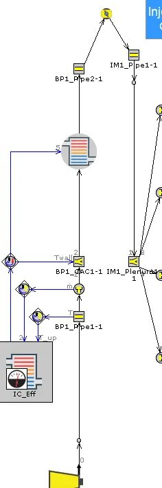
The heat exchanger connection ensures the intercooler outlet temperature. The connection for predictive intercooler was deleted during simplification and therefore they were reconnected. An additional connection to the heat exchanger connection part was created to control the fluid-imposed temperature as it can be seen from the figure above.

Intake pipes:

The model is reduced as shown in the figure below after simplifying the intake pipes sub-volume.

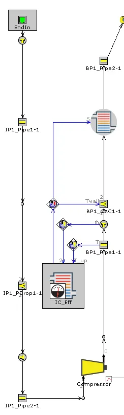
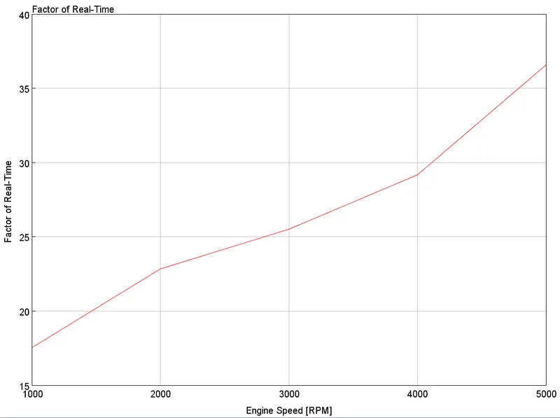
Now, the fast running engine model is complete and the computation time looks as follows:

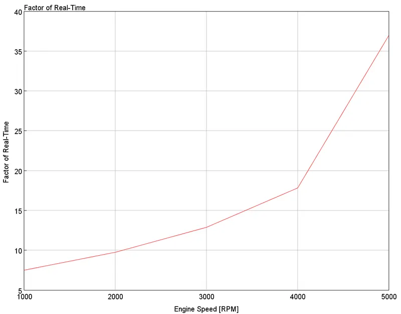
The factor of real-time is around 25 xRT and has high accuracy.

Additional Changes:

The model was further simplified for speed. As it can seen from the figure below, the exhaust manifold still restricts the time-step. Hence a new step was created in the FRM converter and the exhaust manifold sub-volume was selected for simplification. The “Simplify for speed” option was selected here.

The turbine inlet temperature was used as a response variable for the calibration configuration and the heat transfer multiplier of the combined part as the factor variable. The simplified model can be seen in the figure below

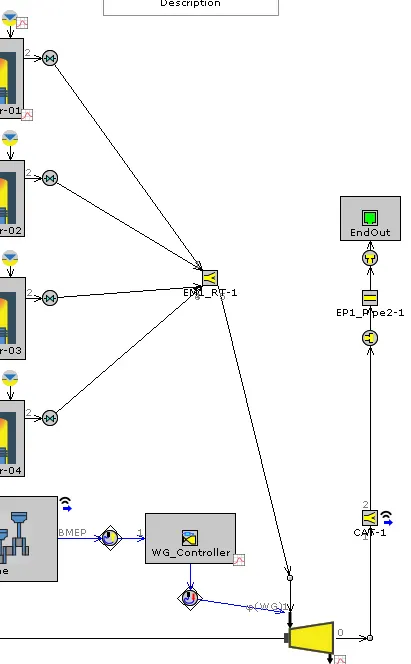
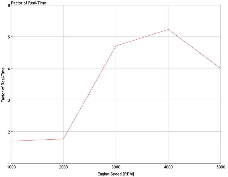
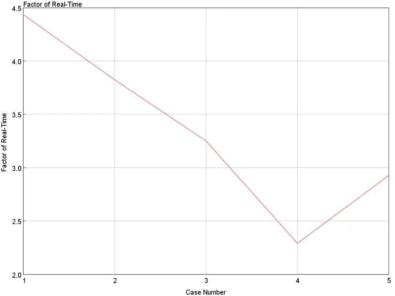
Now the model performance is around 5 xRT as shown in the figure below

Cylinder Slaving:

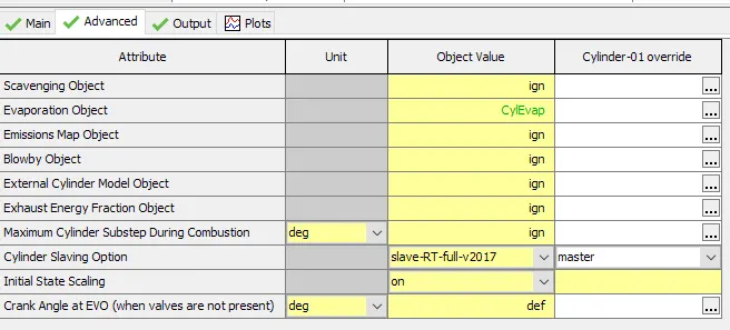
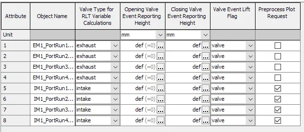
A new step was created in the FRM converter to accomplish this simplification. It is process in which only one cylinder component is solved instead of the all the cylinders. For this, the cylinder-01 was chosen as the master and the valves were chosen to be inlet/exhaust as shown in the figure below.

In this step no sub-volume was selected and the case was calibrated for all the 5 cases.

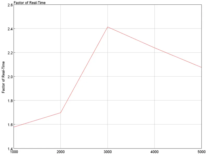
The model performance was improved as shown below.

FRM Builder:

Another option to create a Fast Running Model is to use the FRM Builder option available in GT-Suite. It creates an engine model from a pre-defined set of components and it lacks versatility.

An engine model with the following parameters was created using the FRM Builder option and the resultant model is shown in the following figure.

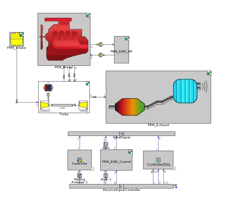
The engine configurations are as follows:

• 6 cylinder CI engine
• Twin-scroll turbine
• Bore=102mm, Stroke=115mm, Compression Ratio = 17
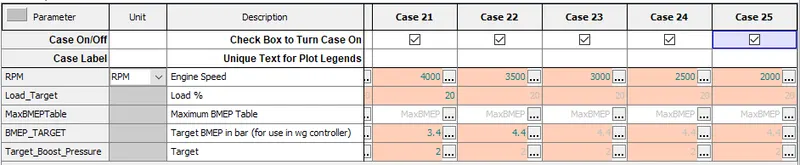
• GT controller

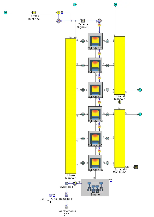
The engine model is shown below. This template uses the cylinder slaving by default. All the controls are handed by wireless signals.

Engine model:

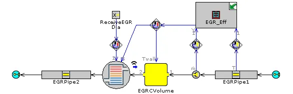
EGR model:

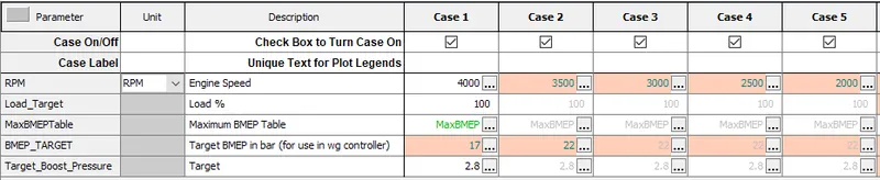
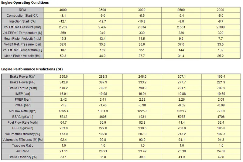
Results:

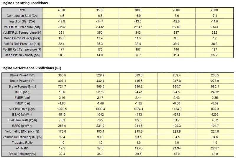
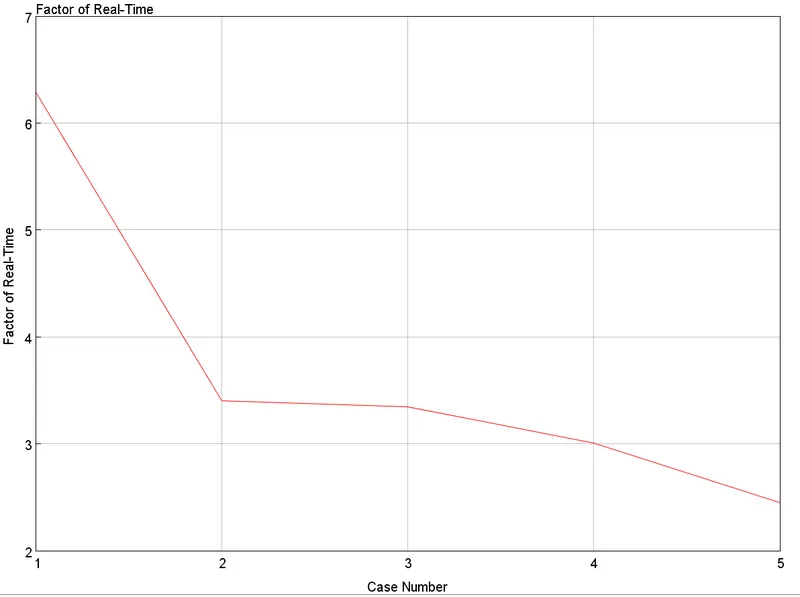
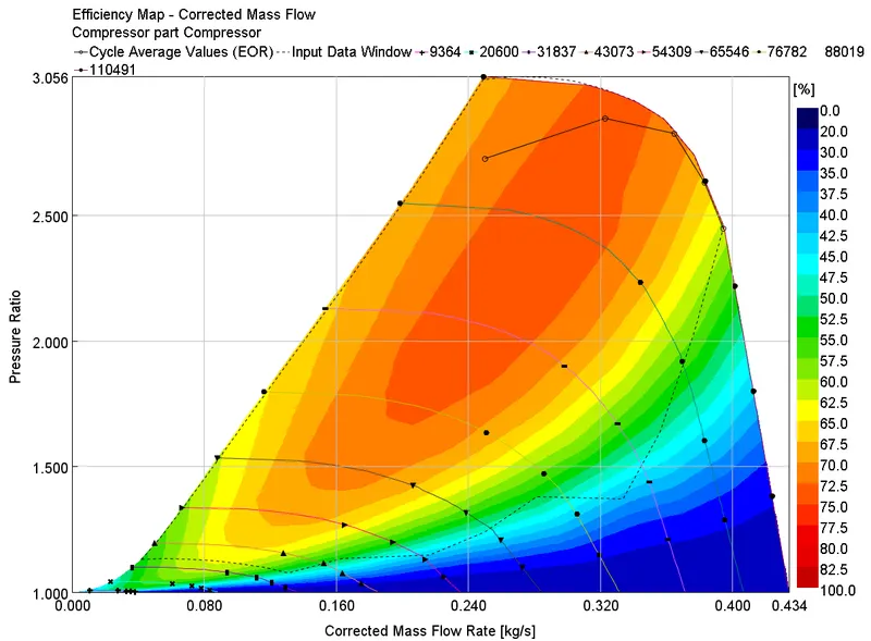
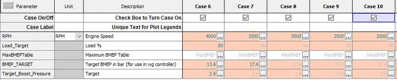
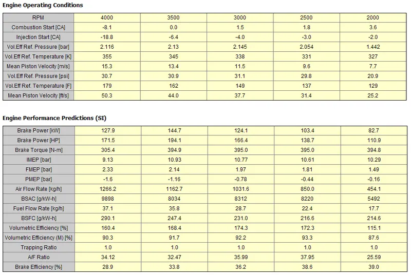
Cases 1 – 5:

Cases 6 -10

Cases 11 – 15

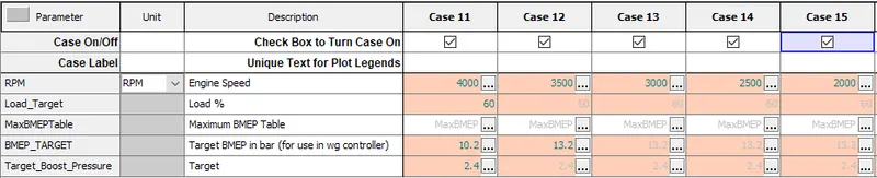
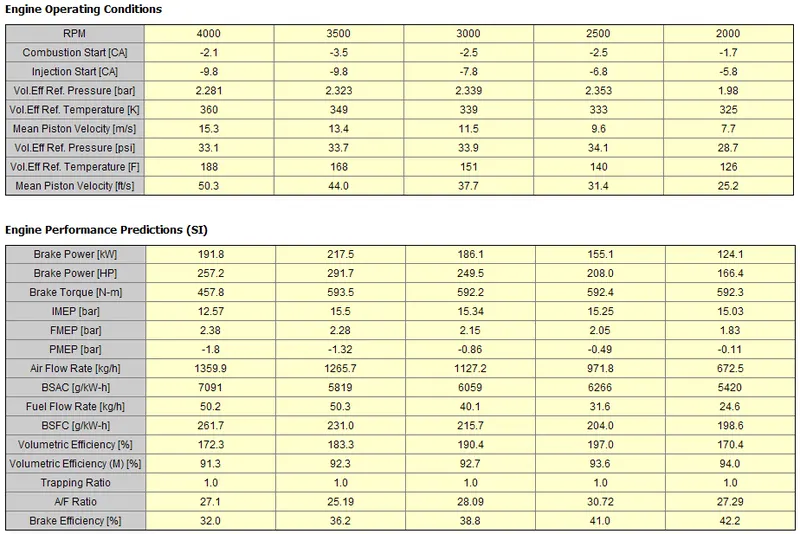
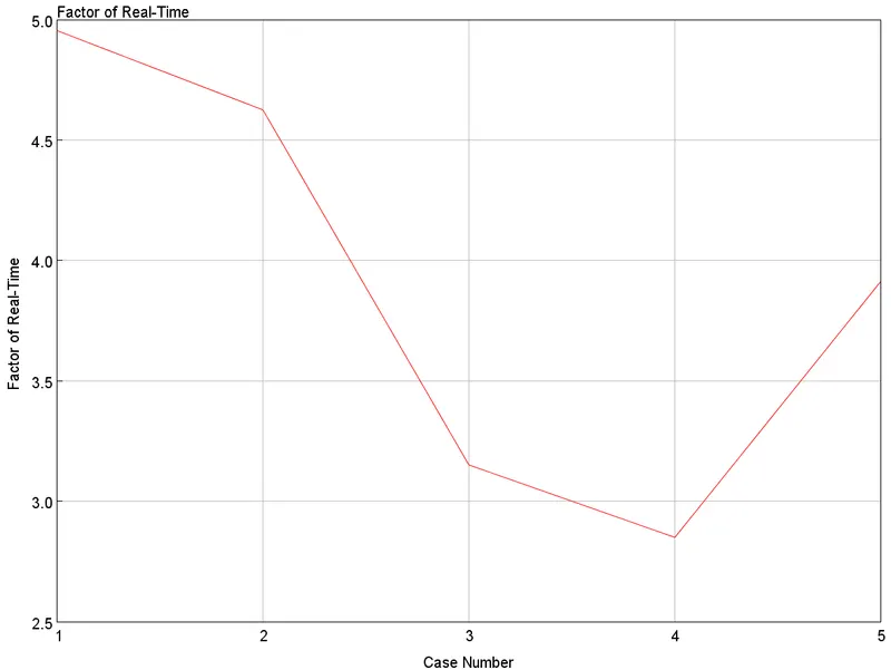
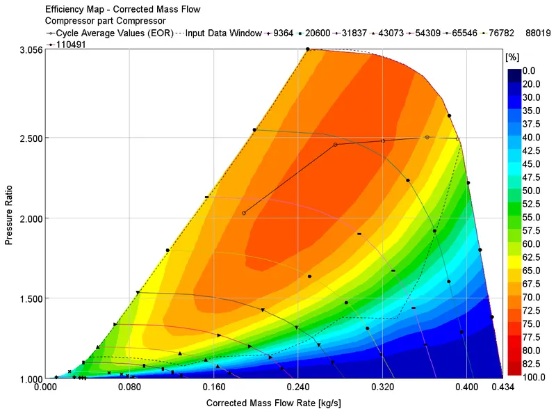
Cases 16 – 20

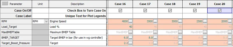
Cases 21 – 25

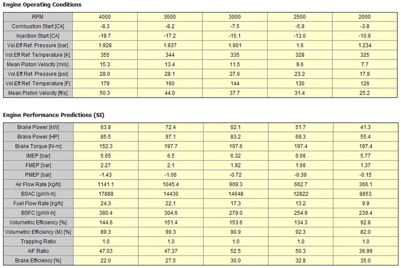
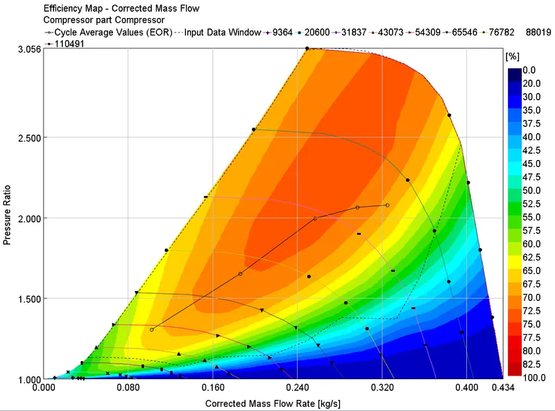
Conclusion:

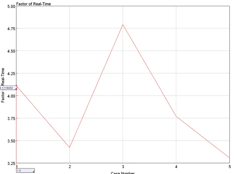
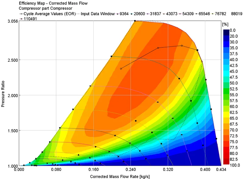
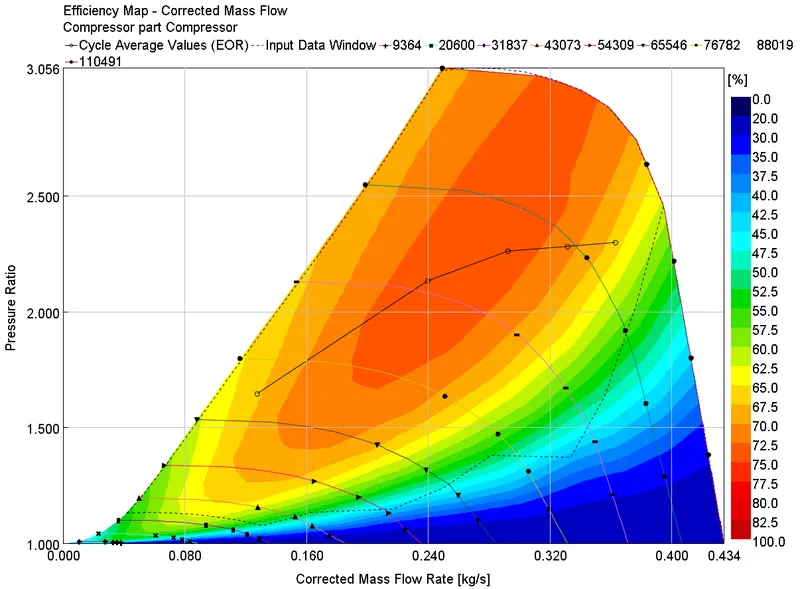
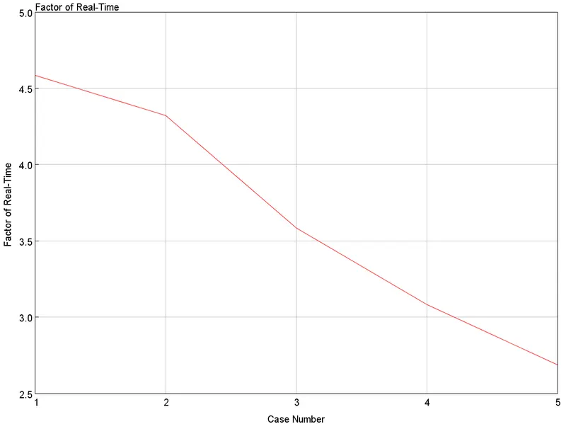
The two FRM options were studied in detail and models were created to test the capabilities. It can be observed from the figures that the FRM builder model had a simulation time of around 5 xRT. It is in comparison to the one achieved by converting the detailed model manually. Although the compressor performance of some of the cases is at the choke line. Hence care should be taken to avoid that.

Comparing the FRM converter and FRM Builder, the latter consumes less time but it lacks flexibility when compared with the former.

References:

1. Gamma Technologies, GT Suite version 2019, ’Engine Performance Tutorials’, Tutorial 9: Building a Fast Running Engine Model (FRM).
2. Fast Running Engine Models (FRMs) for Integrated Simulations (including Real-Time/SiL/HiL) | Gamma Technologies (gtisoft.com)