Week 6 - CHT Analysis on a Graphics card

AIM:

1. To perform steady-state conjugate heat transfer analysis on Graphics Card.
2. To find the effect of different velocities on the temperature.

Objectives:

1. Run the simulation by varying the velocity from 1m/sec to 5m/sec for at least 3 velocities and discuss the results.
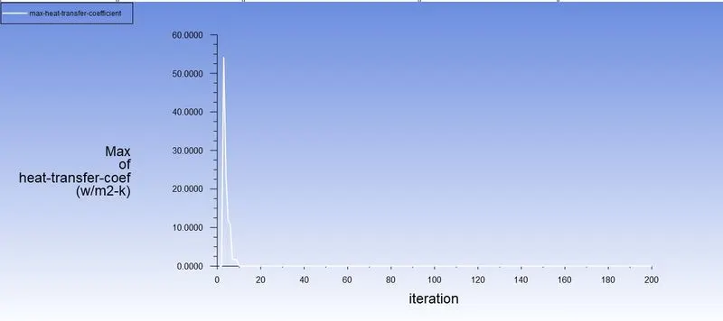
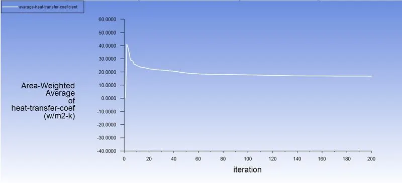
2. Find out the maximum temperature and heat transfer coefficient attained by the processor.
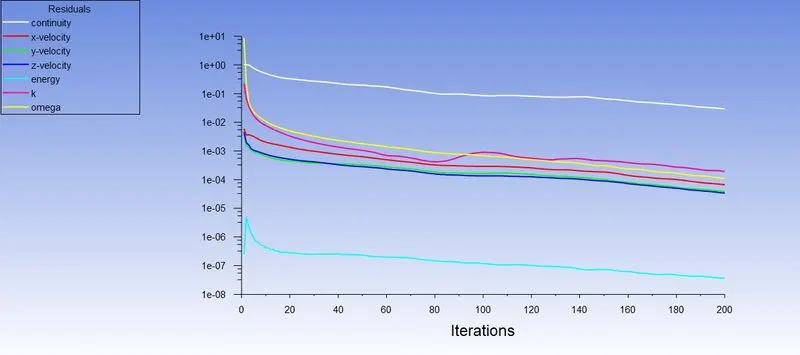
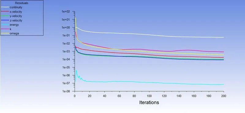
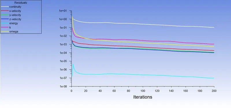
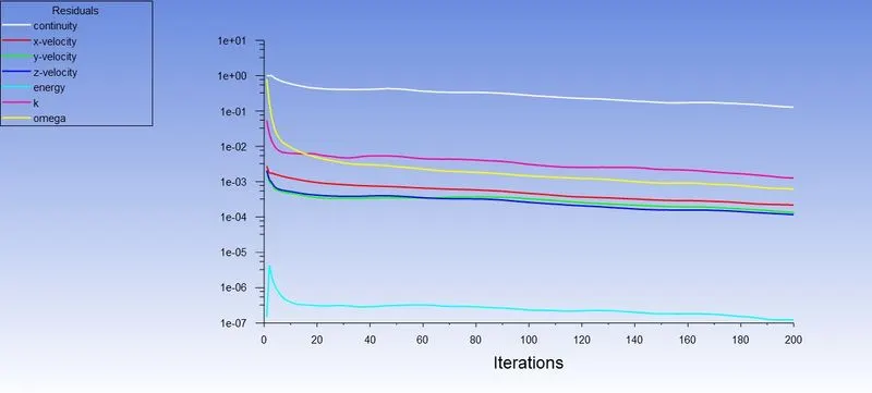
3. Prove that the simulation has achieved convergence with appropriate images and plots.
4. Identify potential hotspots on the model.

Introduction:

In this project , A steady state conjugate heat transfer analysis on a Graphic card has become an everyday used object and a very important part of any computer system , laptops etc. This product is mass produced daily in millions and has made computers exceptionally efficient . As they consume electricity to operate and running a heavy software or graphically task on computer takes a payable use on its graphic card , because of which it generates a large amount of heat .

There is a limit to any system that can hold heat to keep its parts under safe operating condition . We cannot go past these limits as it will damage the system ,Cause failure of the product and system etc. But what we can do is measure to cool this system , cool the graphic card so the system keeps running at optimum speed & condition .

There are various methods of cooling electrical components , through fan , thermal pastes and gels , double fanning , using materials that help dissipating the heat in the fan’s direction , arrangements of components etc.

Cooling of graphic card , i.e. by conduction in the PCB base & fins convection with the surrounding air by providing cooling fins over heat source (graphic card processor) which in turn try to remove heat through conduction and additional air is allowed to flow through assembled components which act as a phenomenon called forced convection.

In this simulation conjugate heat transfer analysis is done on graphic card model by applying heat on the processor of the graphic card while it contained in an enclosure . The air is passed at a certain velocity through the enclosure and we observe the heat dissipation through the fins by conduction from the processor , then observe how the flowing air cools the fins & observe the heat transfer taking place through it.

1. Conjugate Heat Transfer (CHT):

Conjugate heat transfer is defined as the heat transfer between two domains by exchange of thermal energy. For a system the thermal energy available is defined by its temperature and the movement of thermal energy is defined by its heat flux through the outer walls. Heat transfer in solid happens through conduction and walls by convection and in liquid phase through convection.

CHT provides the temperature prediction and the hotspot regions at the solid-fluid interface and we can also predict the heat transfer accurately for example- Conduction through solids, convection through fluid, and thermal radiation. It also provides the velocity and pressure distribution of fluid moving inside the solid. We can also use CHT in design optimization for improvement for heat transfer and cooling capacity.

2.Graphics card:

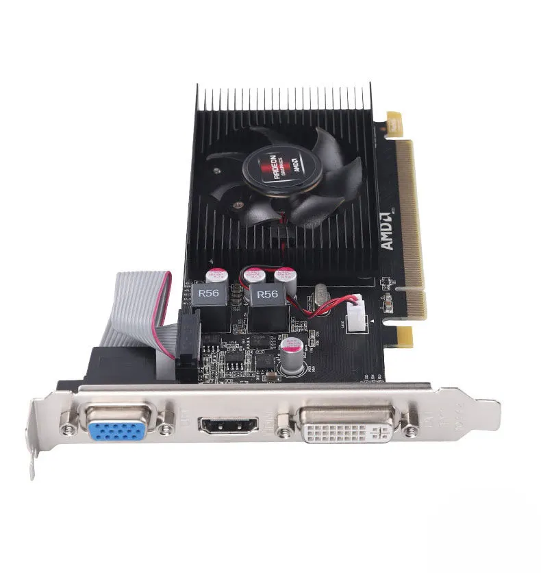
A video card (also called a graphics card, display card, graphics adapter, or display adapter) is an expansion card that generates a feed of output images to a display device (such as a computer monitor). Most video cards are not limited to a 6-inch simple output. Their integrated graphics processor can perform additional processing, removing this task from the central processor of the computer.

Workbench Setup

In this study, a total of 5 simulations was simulated. The first one was the baseline simulation for getting a rough idea and results for the further final simulations.

The next two simulations were performed to check the mesh dependency of the problem setup.

The last two cases were performed to run simulations for different velocities to get study how final results affect by velocity variation.

1.Baseline Mesh - 1m/s -velocity

2. Mesh Dependency check - 1m/s - velocity

3. Mesh Dependency check - 1m/s - velocity

4. Velocity variation - 3m/s - velocity

5. Velocity variation - 5 m/s -velocity

QUESTION:

1. Run the simulation for best possible mesh with combination of coarse and refined mesh in different regions. Explain the reason for choosing the particular mesh settings.

1. First choose Baseline Mesh and find Result....

Baseline Mesh - 1m/s -velocity

PROCEDURE :

1. Geometry

2. Meshing

3.Setup solution

4. Result

1.Baseline Mesh - 1m/s -velocity

1.1 Geometry:

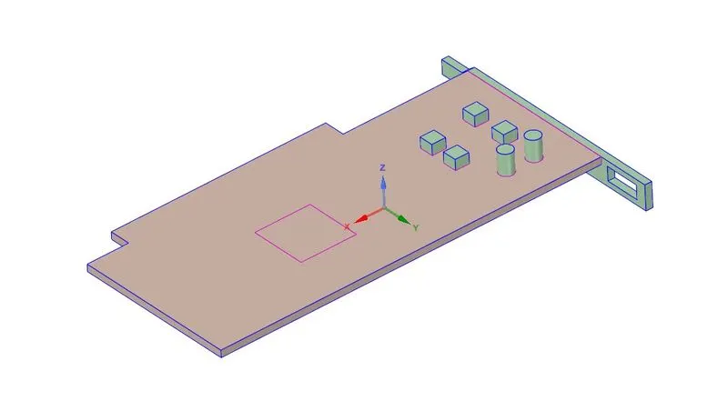
Base:

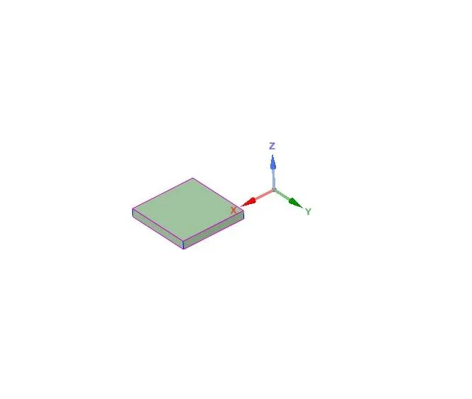
Processor:

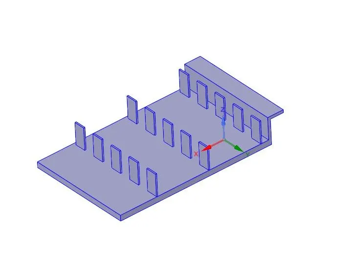
Fins Base:

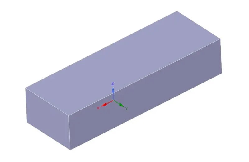
Enclosure:

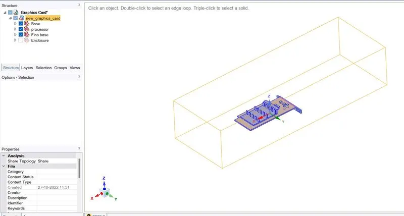
Share topology :

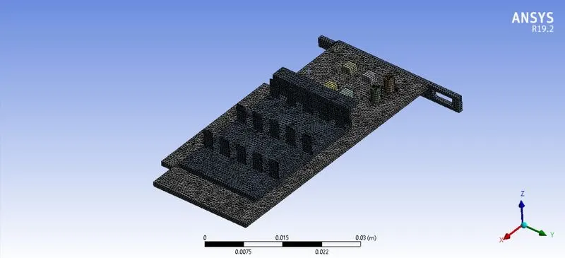
1.2 - Meshing:

After Finishing geometry , the first step is create the name in each geometry faces,

Name selection:

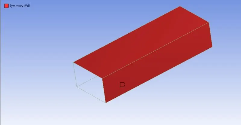
Symmetry Wall:

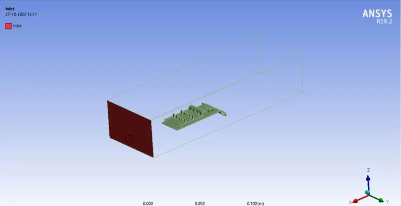
Inlet:

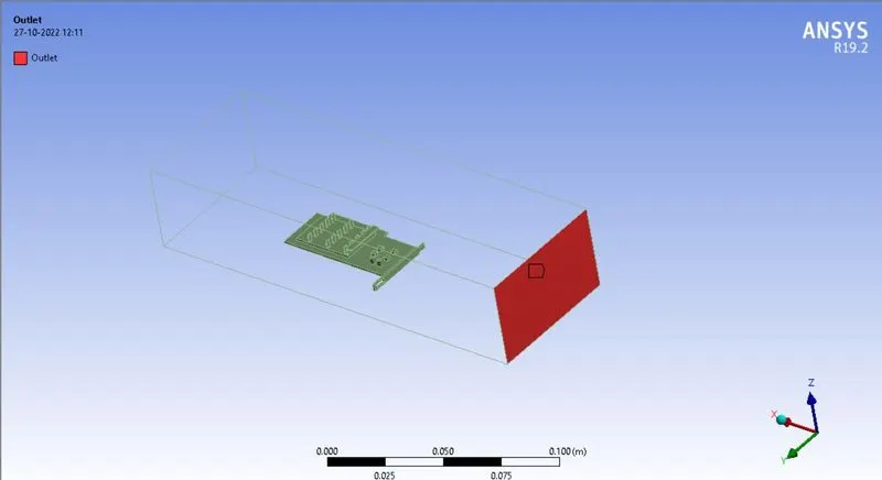
Outlet:

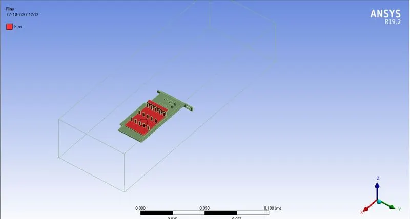
Fins:

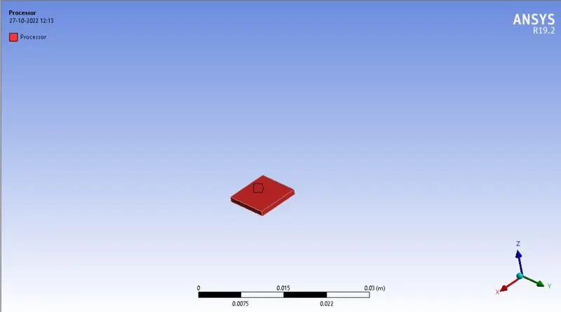
Processor:

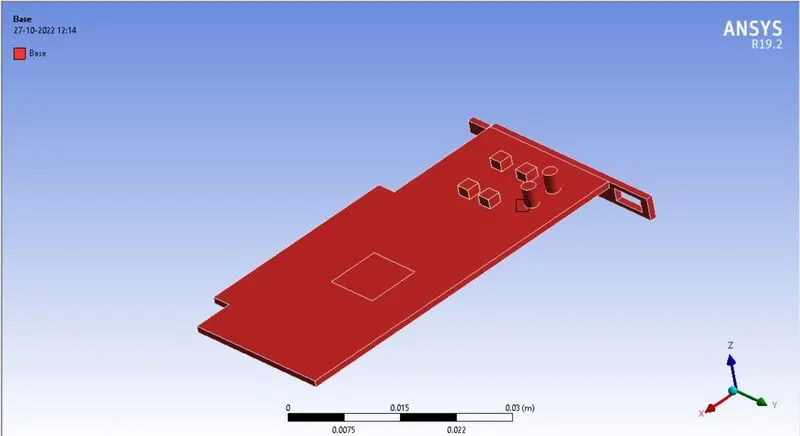
Base:

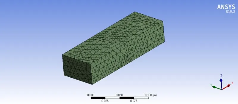
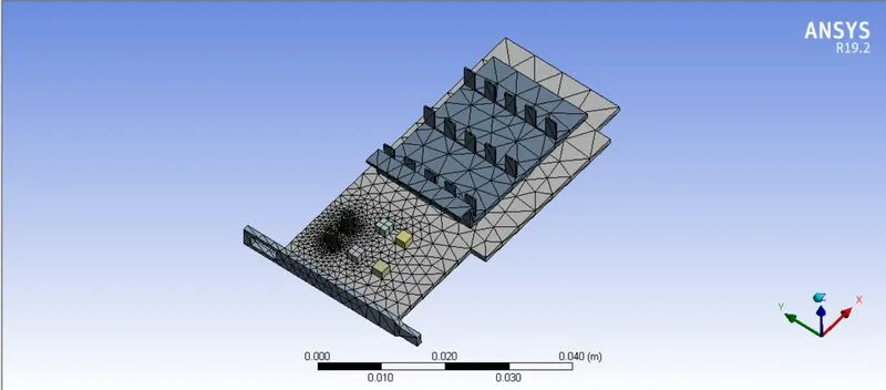
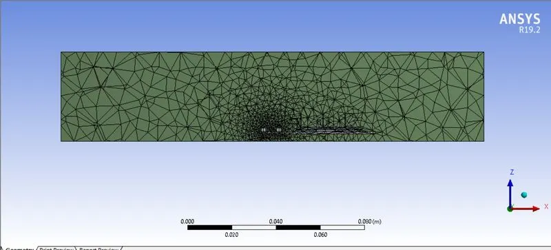
Base Mesh:

A basic mesh is generated using the standard values recommended by Ansys. This mesh is used to obtain an initial solution which will help us to determine the location where mesh refinement is required.

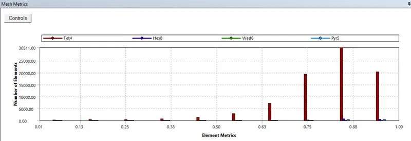
Element Quality:

Mesh settings:

Global mesh setting of element size = 10 mm

1) PCB body sizing

element size = 1 mm
capture curvature - yes, 18 deg

2) Processor body sizing
element size = 1 mm
capture curvature - no

3) fins body sizing
element size = 1 mm
capture curvature - no

1.Element Order: Linear

2.Element size: Default

3.Number of Nodes: 37713

4.Number of Elements: 188843

Fluent Setup:

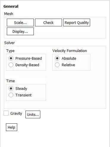
1.Solver: Steady

2.Type: Pressure Based

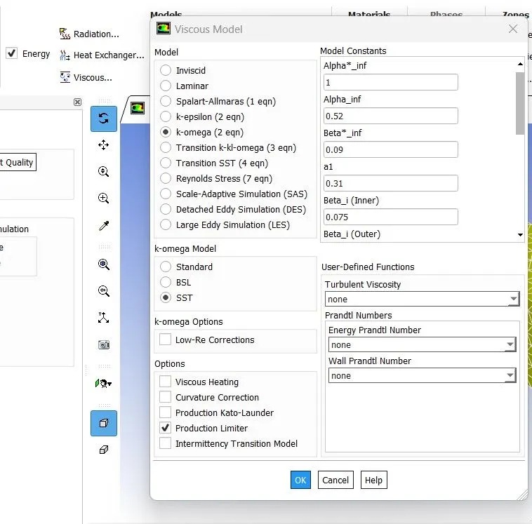
3.Turbulence Model: k-Omega(SST)

4.Materials: Different materials are used for each part, some of which are custom created

• In this particular simulation, the temperature must be calculated so the energy equation needs to be enabled.
• For this simulation, the k-omega turbulent model is considered which is best used for near-wall treatment. This is vital for this simulation as we expect the heat transfer coefficient calculated on the surfaces.
• From the K-omega model, SST was selected as it provides a better prediction of flow separation than most RANS models and also accounts for its good behavior in adverse pressure gradients. It has the ability to account for the transport of the principal shear stress in adverse pressure gradient boundary layers. It is the most commonly used model in the industry given its high accuracy to expense ratio.

Material Selection :

we have created and added 3 solids and 1 fluid for the geometry

1. Fins = Aluminum

2. Processer = Silicon

3. PCB = FR4

4. Fluid = Air

Materials & their properties:

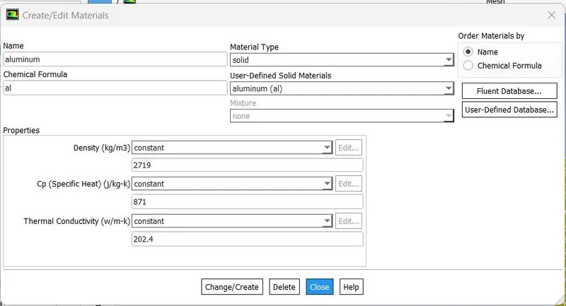
1) Fins --> Aluminum

Standard aluminum is available in Fluent database.

Density = 2719 Kg/m^3

Heat capacity = 871 J/Kg K

Thermal conductivity = 202.4 W/m K

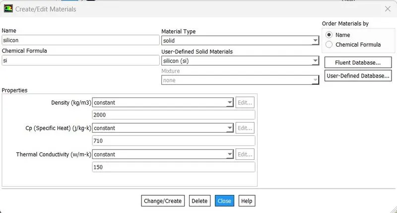
2) Processer --> Silicon

Since the silicon is not available in Fluent's solid database, I had to define it

Density = 2000 Kg/m^3

Heat capacity = 710 J/Kg K

Thermal conductivity = 150 W/m K

3) PCB --> FR4 (glass-reinforced epoxy laminate material)

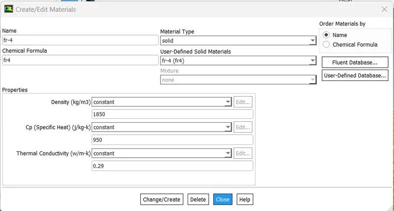
Since the FR4 is not available in Fluent's solid database, I had to define it

Density = 1850 Kg/m^3

Heat capacity = 950 J/Kg K

Thermal conductivity = 0.29 W/m K

4) Fluid --> Air

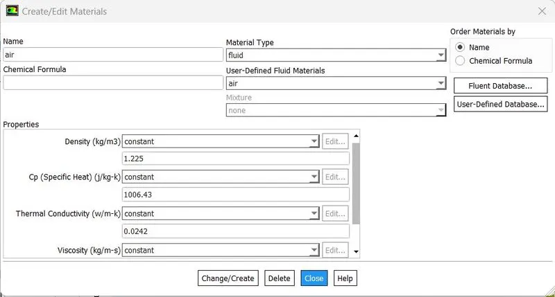
Standard air is available in Fluent database.

Density = 1.225 Kg/m^3

Heat capacity = 1006.43 J/Kg K

Thermal conductivity = 0.0242 W/m K

Viscosity = 1.7894e-05 Kg/m-s

Usually, the power consumed by a processor is converted into heat energy. To calculate the heat generated on the processor which is = Power consumed divided by the total volume of the processor

"The power consumption of today's graphics cards has increased a lot. The top models demand between 110 and 270 watts from the power supply; in fact, a powerful graphics card under full load requires as much power as the rest of the components of a PC system combined"

Heat generation rate = 2.3437e7 W/m^3

Results:

Residuals Polt:

Maximum Heat transfer coefficient:

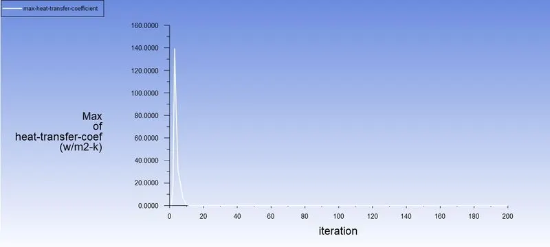
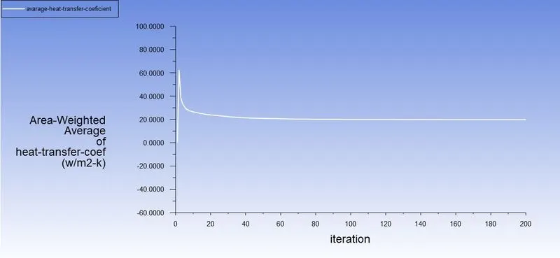
Average Heat transfer coefficient: 19.85 W/m^2 - K

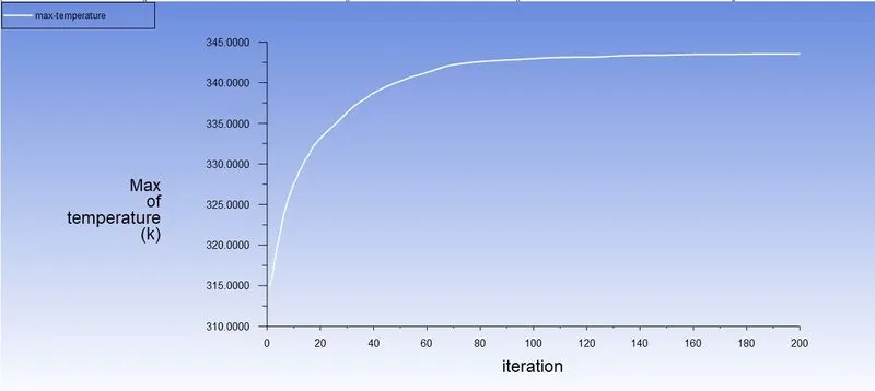
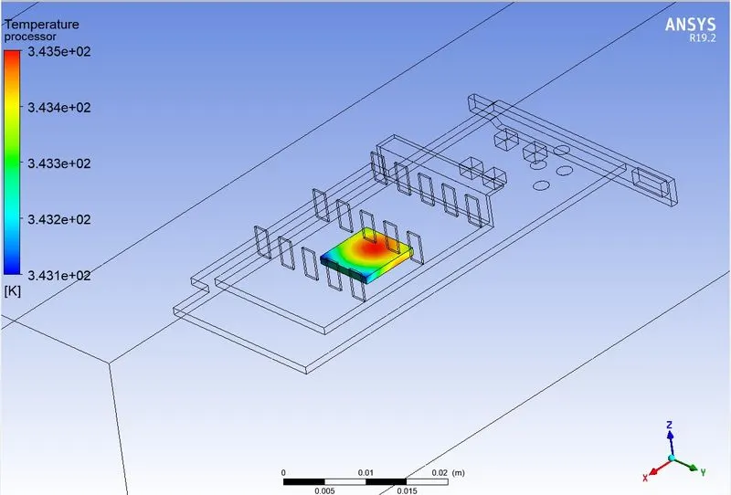
Maximum Temperature in Processor: 343.54 K

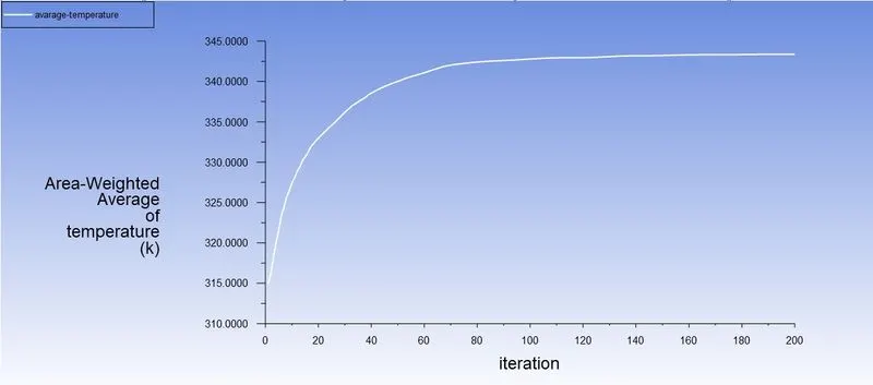
Average Temperature in Processor: 343.36 K

Contour - Temperature - Processor - Global :

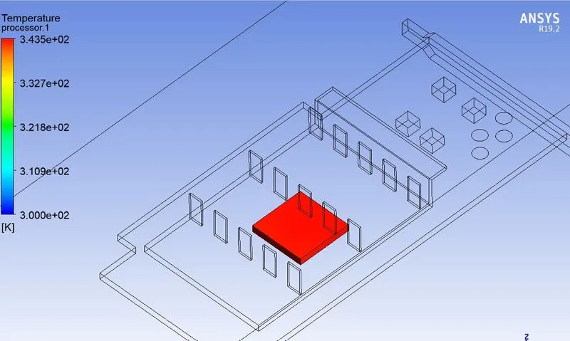
Contour - Temperature - Processor - Local :

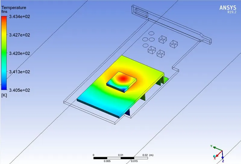
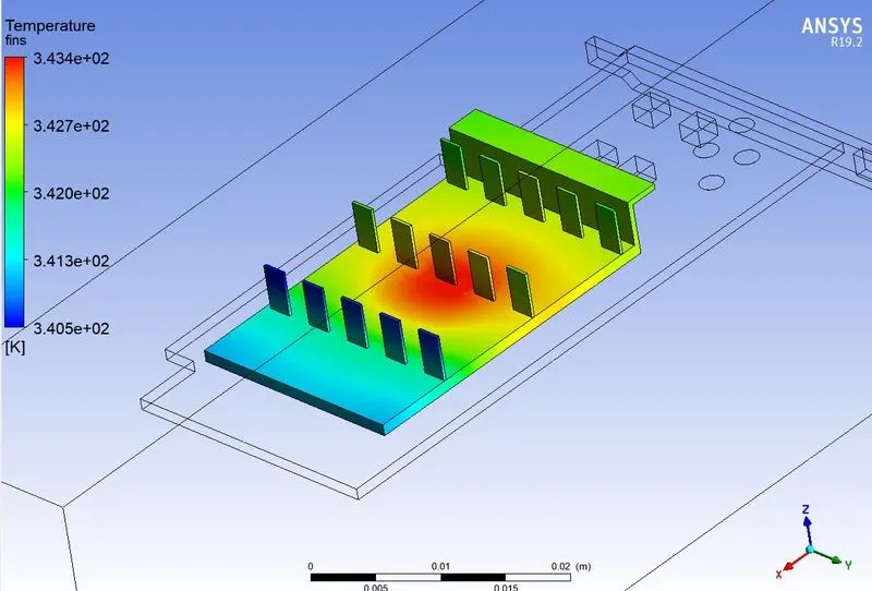
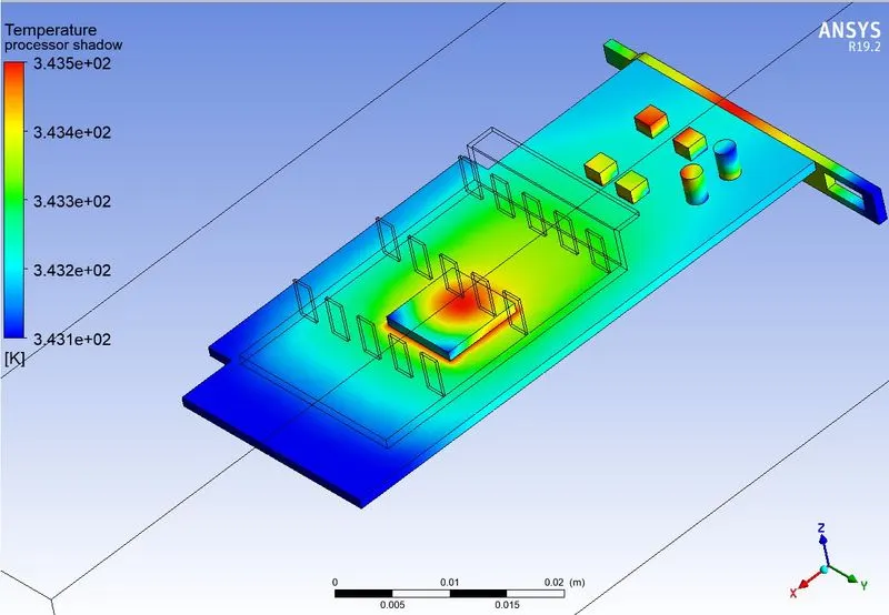
Contour - Temperature - Local :

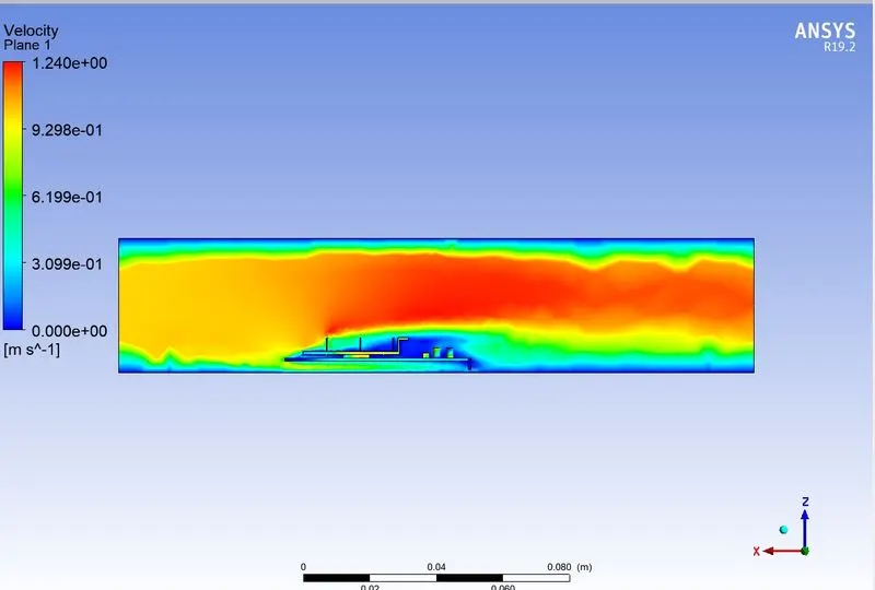
Velocity- contour-plane 1 :

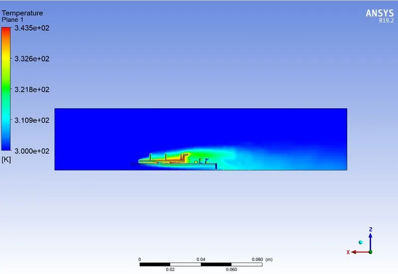
Temperature - Contour -Plane 1 :

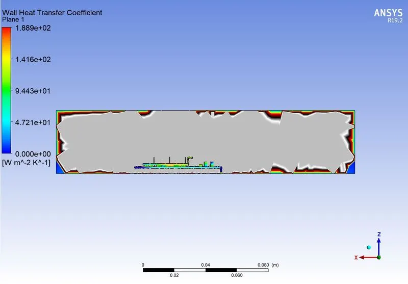
Contour - Wall heat transfer coefficient - Plane 1:

2. REFINED MESH

Velocity:1 m/s

A. MESH

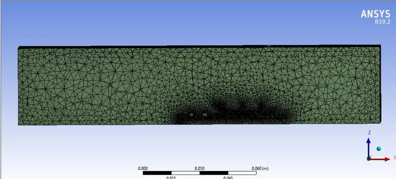
1.Element Order: Linear

2.Element size: 0.003 m

3. Body Sizing (Fin)

• Element Size: 0.0005 m
• Curvature Capture: Yes

4. Body Sizing (Processor)

• Element Size: 0.0005 m
• Curvature Capture: Yes

5. Body Sizing (Base)

• Element Size: 0.005 m
• Curvature Capture: Yes

6.Number of Nodes: 154622

7.Number of Elements: 796057

Meshing:

Results:

Residuals Polt:

Maximum Heat transfer coefficient:

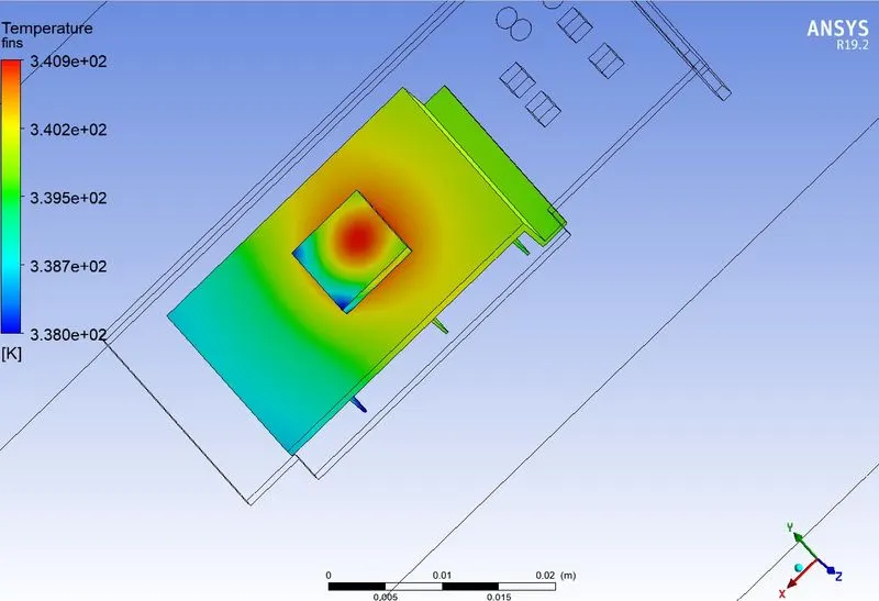
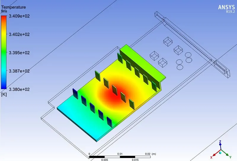
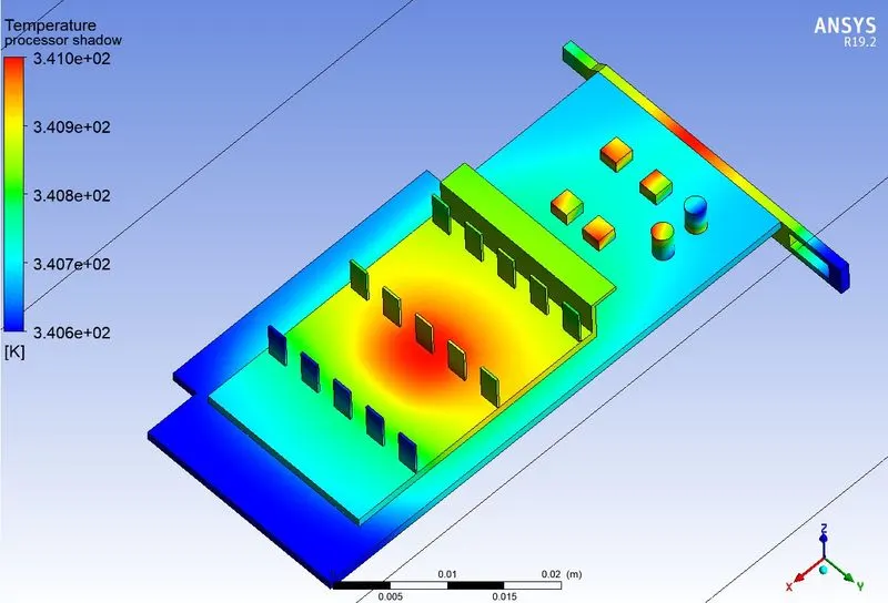
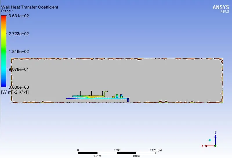
Average Heat transfer coefficient: 16.768 W/m^2 - K

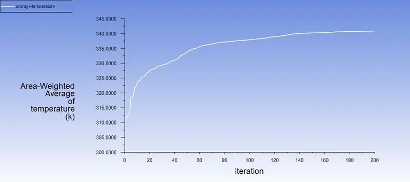
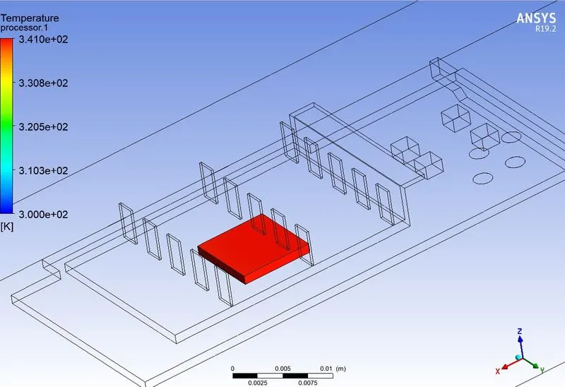
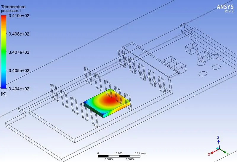
Maximum Temperature in Processor: 341.0358 K

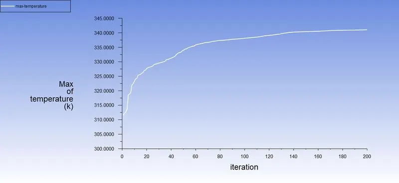
Average Temperature in Processor: 340.852 K

Contour - Temperature - Processor - Global :

Contour - Temperature- Processor - Local :

Contour - Temperature - Local :

Velocity- contour-plane 1 :

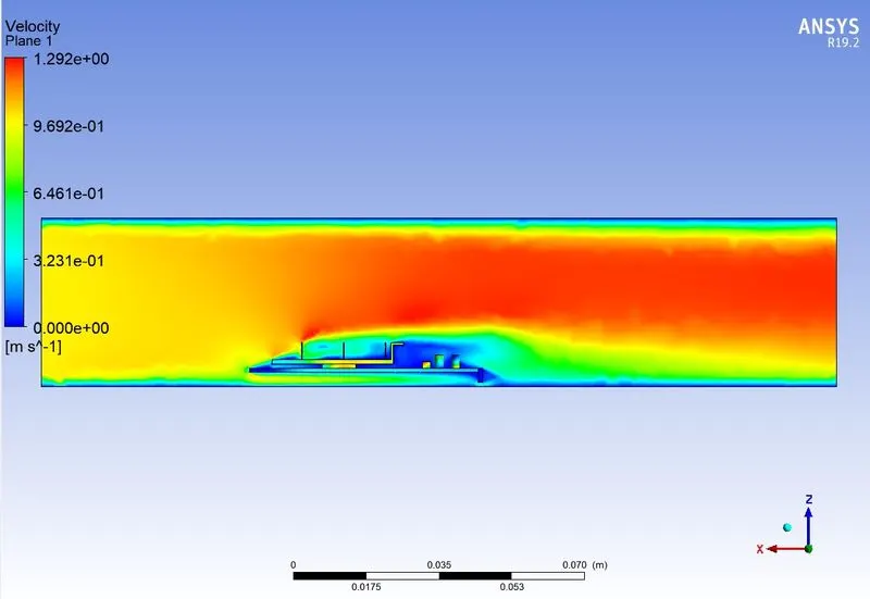
Temperature - Contour -Plane 1 :

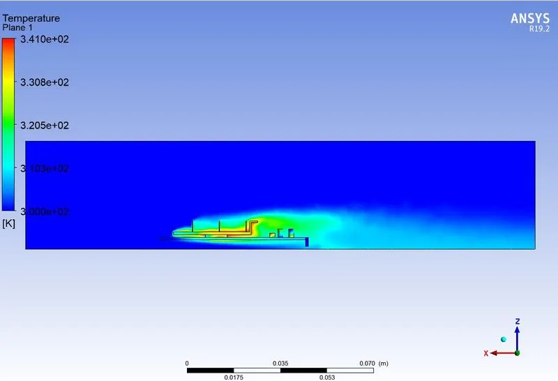
Contour - Wall heat transfer coefficient - Plane 1:

3.

• Now the Refined Mesh is more accurate in compared to base mesh, Hence we choose mesh in refined type of mesh for next different velocity simulation .
• Already velocity 1m/s Refined mesh simulation is completed, so we going to do other velocity of 3m/s and 5 m/s choose refined mesh

4. Velocity: 3m/s

Meshing : 2. Refined Mesh

Results:

Residuals Polt:

Maximum Heat transfer coefficient:

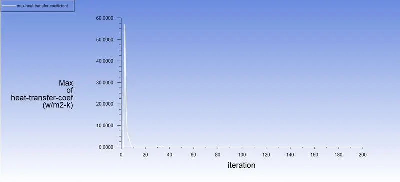
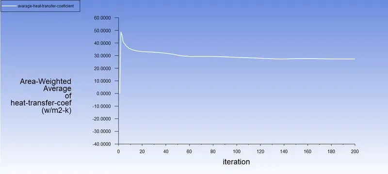
Average Heat transfer coefficient: 27.344 W/m^2 - K

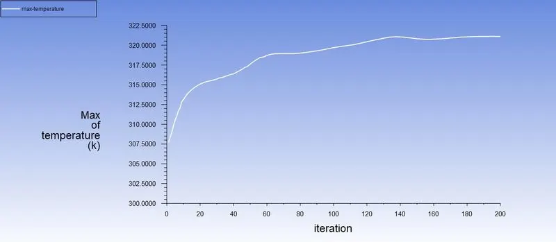
Maximum Temperature in Processor: 321.1028 K

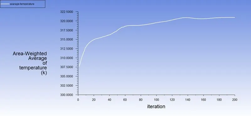
Average Temperature in Processor: 320.928 K

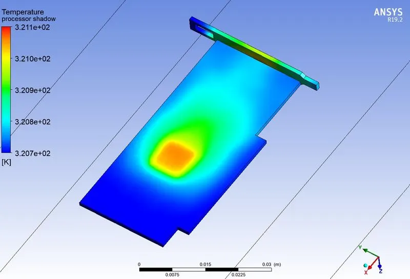
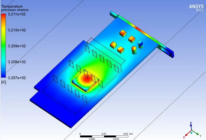
Contour - Temperature - Processor - Global :

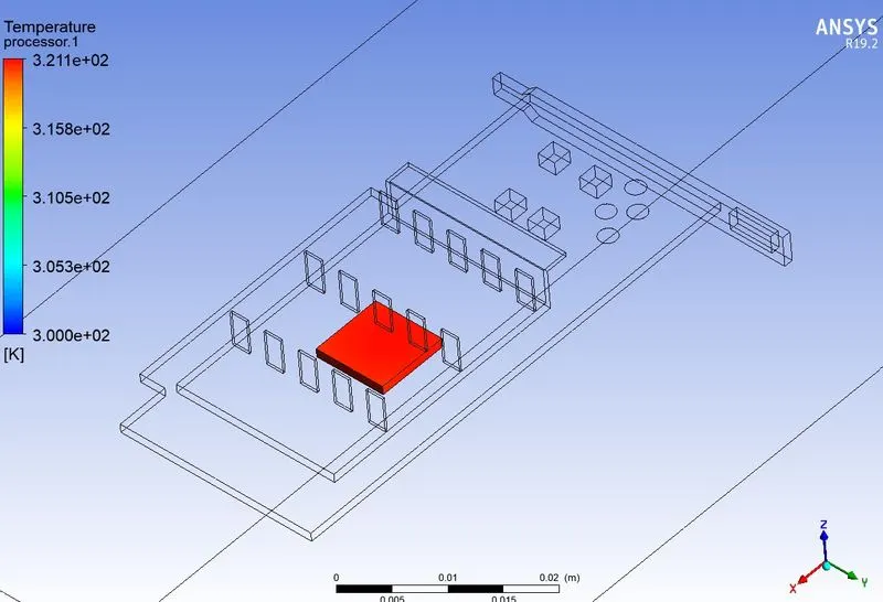
Contour - Temperature - Processor - local :

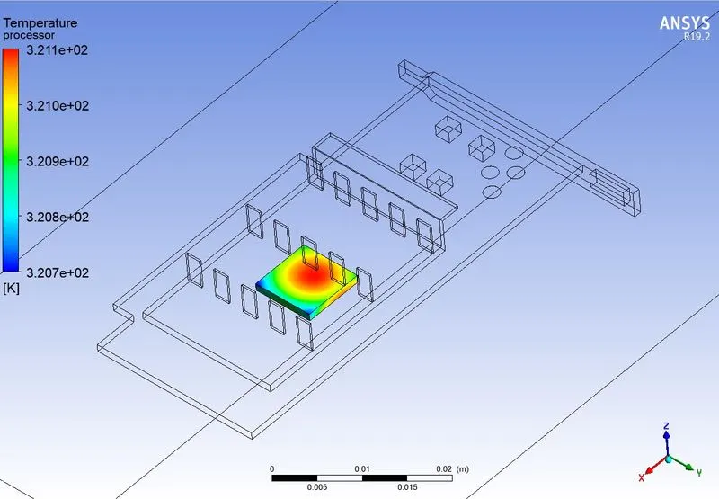
Contour - Temperature - Local :

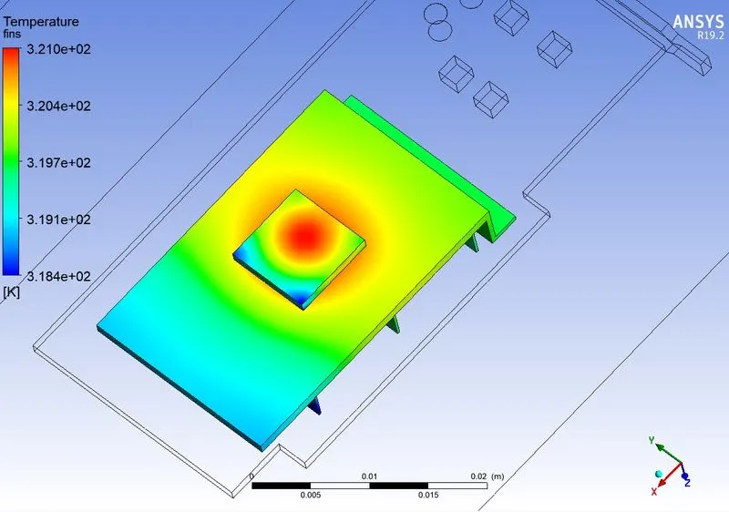
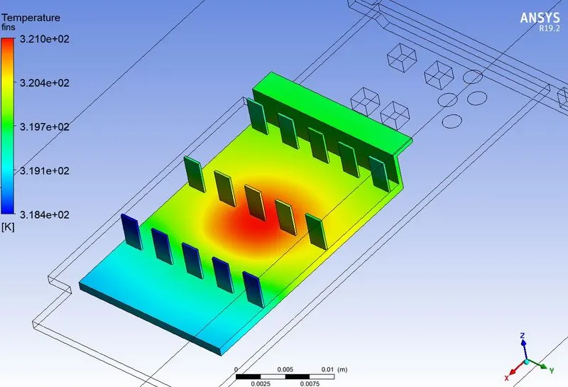
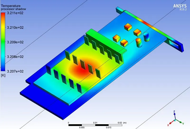
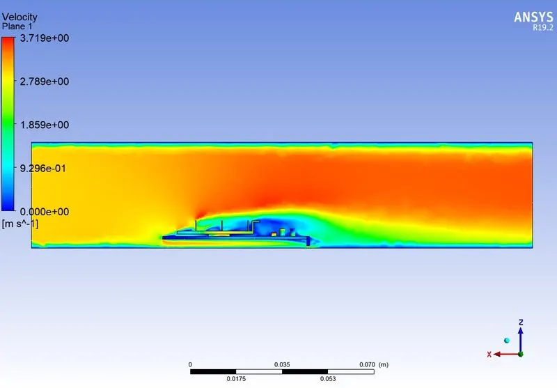
Velocity- contour-plane 1 :

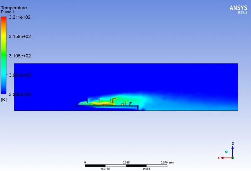
Temperature - Contour -Plane 1 :

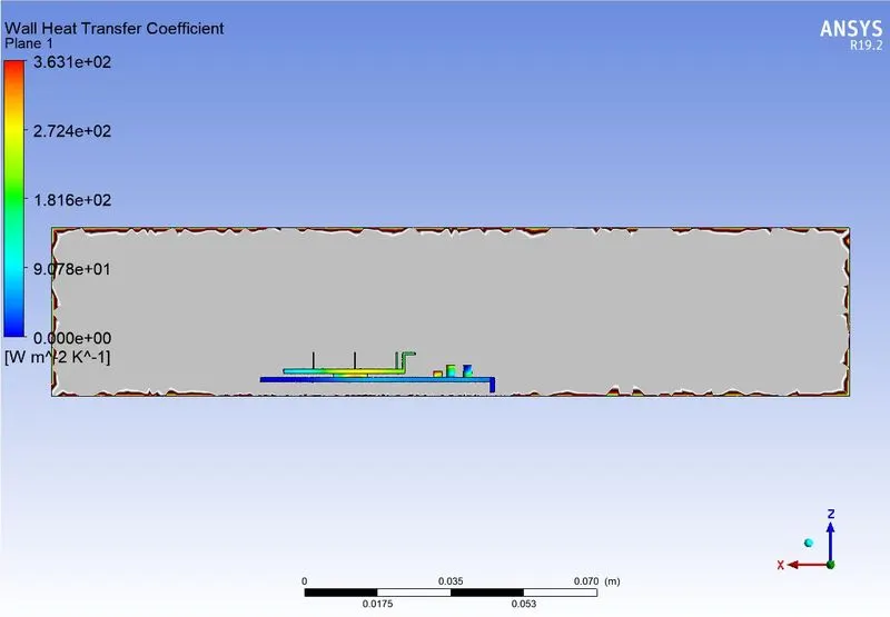
Contour - Wall heat transfer coefficient - Plane 1:

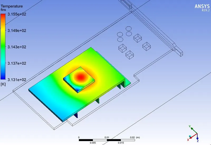
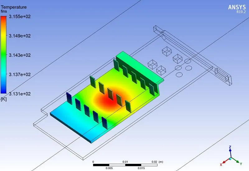
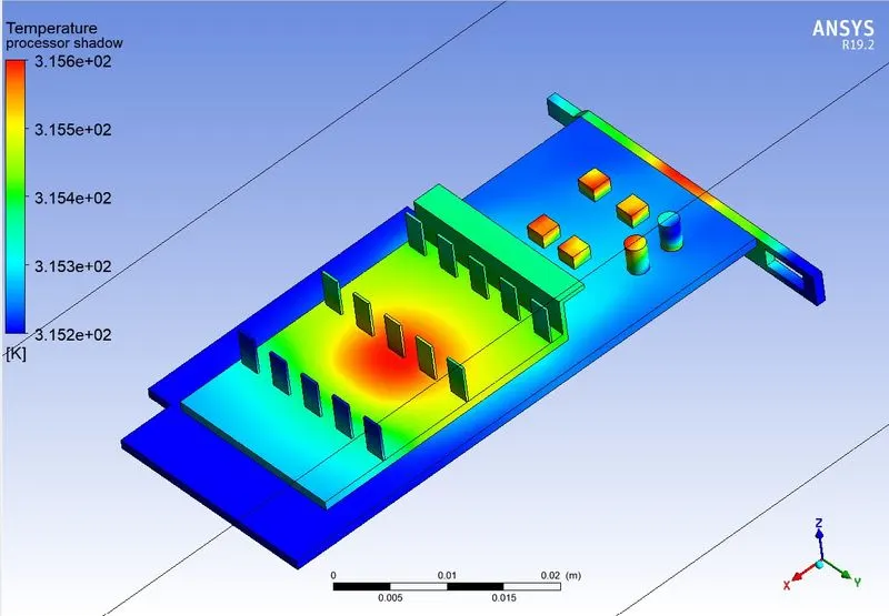
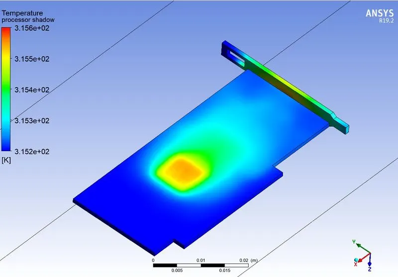
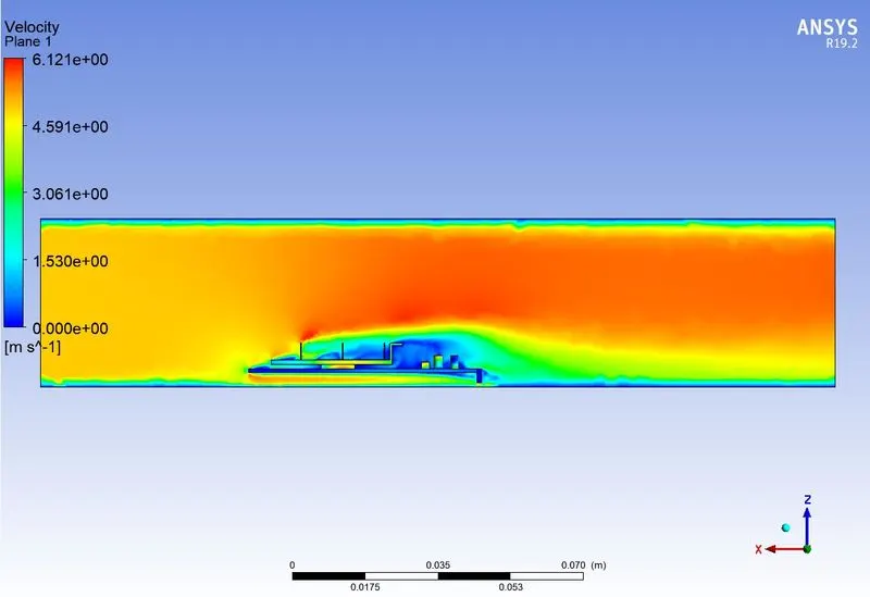
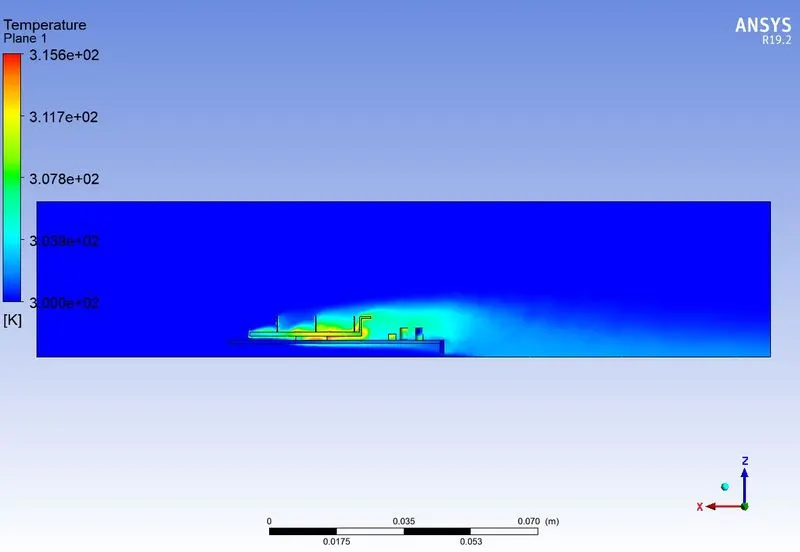
5. Velocity: 5m/s

Meshing : 2. Refined Mesh

Results:

Residuals Polt:

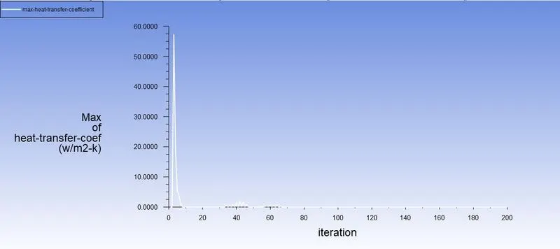
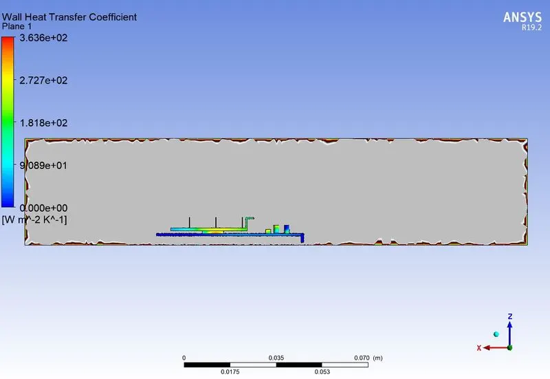
Maximum Heat transfer coefficient:

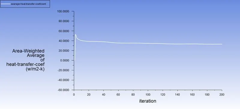
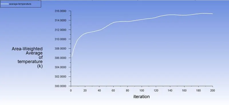
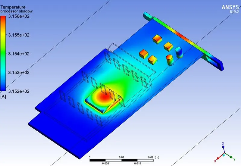
Average Heat transfer coefficient: 33.081 W/m^2 - K

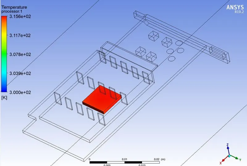
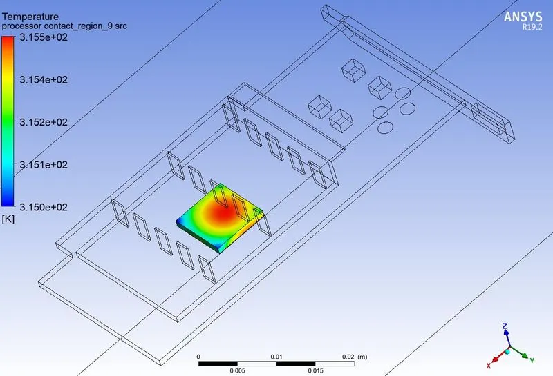
Maximum Temperature in Processor: 315.587 K

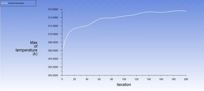
Average Temperature in Processor: 315.414 K

Contour - Temperature - Processor - Global :

Contour - Temperature - Processor - local :

Contour - Temperature - Local :

Velocity- contour-plane 1 :

Temperature - Contour -Plane 1 :

Contour - Wall heat transfer coefficient - Plane 1:

Final Output Results:

Mesh	Velocity	Nodes	Elements	Max. Temp -Processor (K)	Avg. Temp -Processor (K)	Max. HTC (W/m^2 - K)	Avg. HTC (W/m^2 - K)
Baseline Mesh	1 m/s	37713	188843	343.54	343.36	62	19.85
Refined Mesh	1 m/s	154622	796057	341.0358	340.852	54.5	16.768

Mesh	Velocity	Nodes	Elements	Max. Temp -Processor(K)	Avg. Temp -Processor (K)	Max. HTC (W/m^2 - K)	Avg. HTC (W/m^2 - K)
Refined Mesh	1 m/s	154622	796057	341.0358	340.852	54.5	16.768
Refined Mesh	3 m/s	154622	796057	321.102	320.928	57	27.34
Refined Mesh	5 m/s	154622	796057	315.587	315.44	56.3	33.081

Conclusion:

1. As the number of elements increases the accurate results of temperature distribution is obtained
2. From the above table, it is fairly notable that, the net temperature of components of graphics cards decreases with an increase in inlet velocity.
3. Hence it can be inferred that a higher inlet velocity results in better cooling and lower the average temperature thus keeping the components safe from damage.
4. Furthermore, it can be observed that the temperature of components increases as the inlet velocity decreases from 5 m/s to 1m/s, also proving that higher velocity results in better cooling.