Week 6 - CHT Analysis on a Graphics card

Problem Statement: -

Perform a Steady State CHT analysis on the Given Graphic Card Model for 3 inlet Velocities 1 m/sec, 3 m/sec, and 5 m/sec for Course and Fine Mesh. Create an appropriate Mesh, define appropriate Materials for each Component and Perform a mesh-independent Study.

Expected Results: -

1. Explain the Relevant Theories for the CHT Analysis.

2. Generate the Relevant Result Contours and Plots

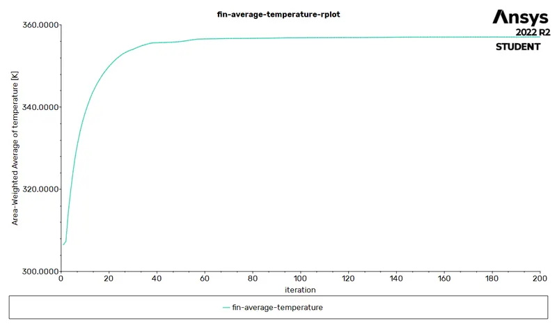
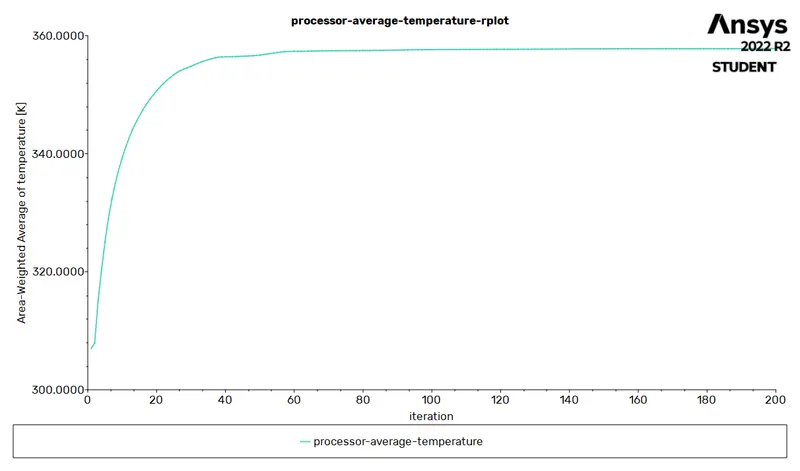
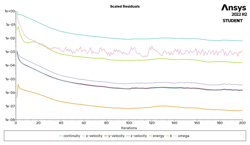
3. Explain the Results and Explain if the result is converged

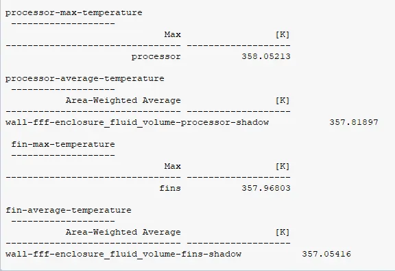
4. Find the Max temperature attained by the Fins and Processor

Solution: -

AIM: -

A. Perform a Conjugate Heat Transfer Analysis on a Graphics Card by selecting appropriate Materials for all the Components.

B. Perform the Analysis for 3 different Velocities and Find the Maximum Temperature and Heat Transfer Coefficient for the Processor.

Given and Assumed: -

A. The CAD Model of the Graphics Card with the Enclosure: -

Graphics Card

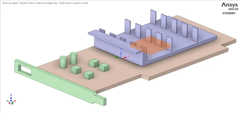Enclosure For Analysis

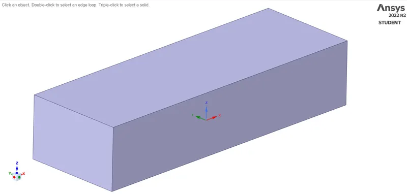B. Materials and their Properties: -

Part/Materials	Density`((kg)/m^3)`	Thermal Conductivity`(W/(m*K))`	Specific Heat Coefficient`(J/(kg*K))`
Processor/Silicon	2329	148	700
Fins/Copper	8978	387.6	381
PCB/FR-4	1850	0.3	1100
Enclosure/Air	1.225	0.242	1006.43

C. Conditions at Different Locations: -

i. Inlet Velocities: -

a. Condition 1 `->` 1 m/sec

b. Condition 2 `->` 3 m/sec

c. Condition 3 `->` 5 m/sec

ii. Outlet Pressure(for any Condition) `->` 101.325 KPa or 1 atm

iii. Power Consumption Rate by Processor `->` 2 W

Measurement of Processor and Density of Heat Generation: -

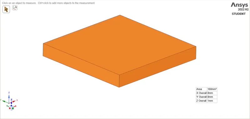The Volume of Processor: -

`=>` Volume = `l*b*h`

`=>` Volume = `8*8*1 m^3`

`=>` Volume = `64 m^3`

The Heat Generation in Processor per unit Volume

`dot(q) = dot(Q)/("Volume")`

`=> dot(q) = 3.125*10^7 W/m^3`

Processor's Heat Generation Rate = `3.125*10^7 W/m^3`

Theory: -

A. Heat Dissipation from Fins: -

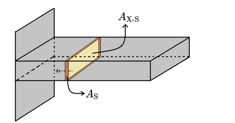
The Extended Surfaces on the exterior of an object that increases the Surface area for Heat Transfer from the Object to the immediate Surroundings are termed Fins. Fins are efficient ways to improve heat rejection from a Surface to the surroundings.

Now,

From Energy Balance,

Energy Entering from Left = Energy Convected + Energy Leaving from Right Side

`=> ubrace(dot(Q)_x)_("Energy Entering From Left") = ubrace(dot(Q)_x + (deldot(Q)_x)/(delx)dx)_("Energy Leaving From Right") + ubrace(dot(Q)_c)_("Energy Released through Convection")`

`=> (deldot(Q)_x)/(delx)dx + dot(Q)_c = 0`

`=> (del)/(delx)(kA_("X-S")(delT)/(delx))dx + h(delA_S)(T_x - T_oo) = 0`

`=> kA_("X-S")(del^2T)/(delx^2)dx + k(delT)/(delx)((delA_("X-S"))/(delx))dx + h(delA_S)(T_x - T_oo) = 0`

`=> k(del^2T)/(delx^2) + k/A_("X-S")(delT)/(delx)((delA_("X-S"))/(delx)) + h/A_("X-S")(delA_S)/(delx)(T_x - T_oo) = 0`

`=> (del^2T)/(delx^2) + 1/A_("X-S")(delT)/(delx)((delA_("X-S"))/(delx)) + h/(k*A_("X-S"))(delA_S)/(delx)(T_x - T_oo) = 0`

Governing Equation for Heat Released by the Fins

`(del^2T)/(delx^2) + 1/A_("X-S")(delT)/(delx)((delA_("X-S"))/(delx)) + h/(k*A_("X-S"))(delA_S)/(delx)(T_x - T_oo) = 0`

B. K-Omega SST Turbulence Model: -

This is a hybrid Model which has the features of the K-Omega and K-Epsilon Turbulence Modeling that uses the K-Omega Model closer to the wall and by switching uses the K-Epsilon Model near the free stream.

Steps to Setup the Conjugate Heat Transfer Analysis of Graphic Card: -

A. Setting up the Ansys Workbench: -

Ansys Workbench `->` ToolBox `->` Analysis System `->` `ubrace("Fluid Flow(Fluent)")_("Selecting" -> "Holding" -> "Dragging and Drooping to Project Schematic")`

B. Opening SpaceClaim Geometry and Sharing Topology: -

i. Steps to Open SpaceClaim: -

Ansys Workbench `->` Project Schematic `->` Project `->` Geometry `->` Right-Click `->` Select SpaceClaim Geometry

ii. Steps to Load the Graphic Card with Enclosure Geometry: -

SpaceClaim `->` File `->` Open

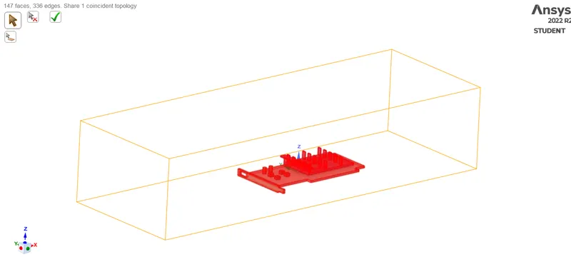
iii. Steps to create Share Topology between the Domains: -

SpaceClaim `->` Workbench `->` `ubrace("Share")_("It will auto-detect the Common Boundaries")` `->` Enter

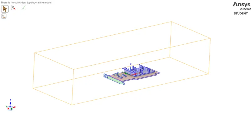Common Area For Sharing	Shared Topology

C. Opening Mechanical(Meshing) and Meshing the Geometry: -

i. Steps to Open Meshing: -

Ansys Workbench `->` Project Schematic `->` Project `->` Mesh `->` Right-Click `->` Edit

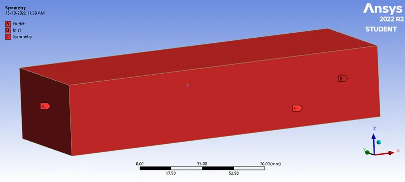
ii. Steps to Name the Boundary: -

Mechanical(Meshing) `->` Model Working Window `->` Select the Boundary `->` Click N `->` Give the desired Name `->` Enter

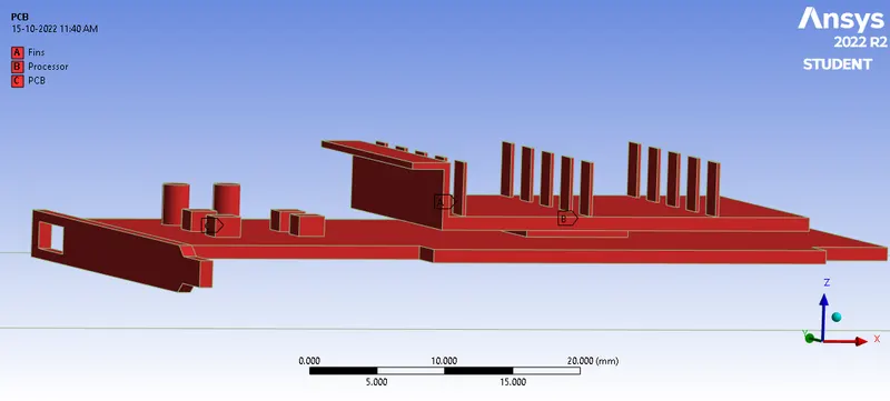Fluid Domain Namings	Solid Domain Namings

iii. Steps to Create the Mesh: -

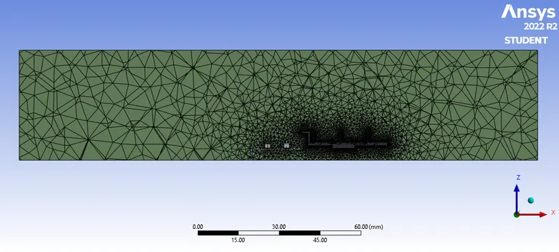
a. Setting Base Mesh Size: Outline Window `->` Select Mesh `->` Details of Mesh Window `->` Defaults `->` Element Size is set to "8mm"

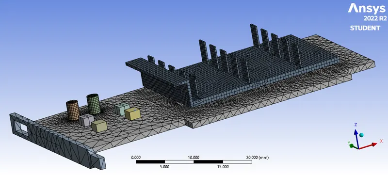
b. Giving Hex Dominant Mesh for Processor and Fins: `ubrace("Select the Desired Geometry")_("Select the Processor and Fins")` `->` Mesh `->` Right-Click `->` Select "Method" from Insert `->` `ubrace("Select the desired Mesh Parameters")_("In our Case for the Selected Geometry Select Hex Dominant")`

c. Giving Mesh Size for Processor and Fins: `ubrace("Select the Desired Geometry")_("Select the Processor and Fins")` `->` Mesh `->` Right-Click `->` Select "Sizing" from Insert `->` `ubrace("Select the desired Mesh Parameters")_("In our Case for the Selected Geometry Define mesh Size as 0.5mm")`

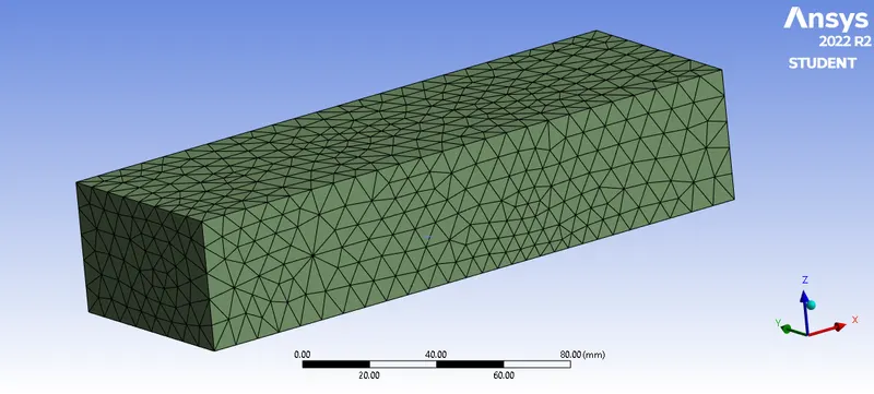Meshed Graphics Card with Hex Dominant Fins and Processor	Meshed Computational Domain
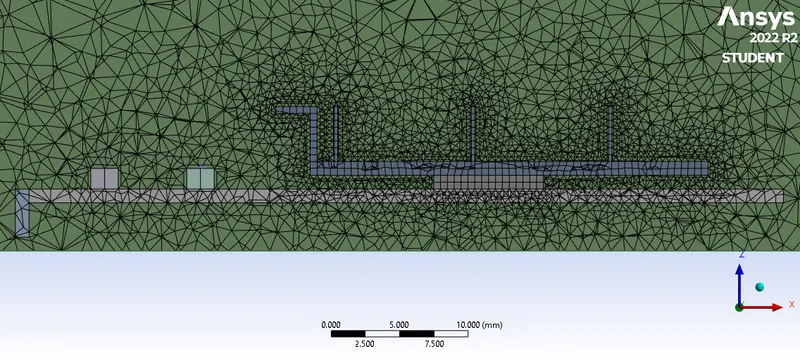Meshed Computational Domain Front View	Meshed Graphics Card and Computational Domain

D. Setuping the Physics and Boundary Conditions: -

i. Steps to Open Ansys Fluent: -

Ansys Workbench `->` Project Schematic `->` Project `->` Setup `->` Right-Click `->` Edit

ii. Steps to Check Mesh: -

Fluent `->` Outline View Window `->` Setup `->` General `->` Mesh `->` Check

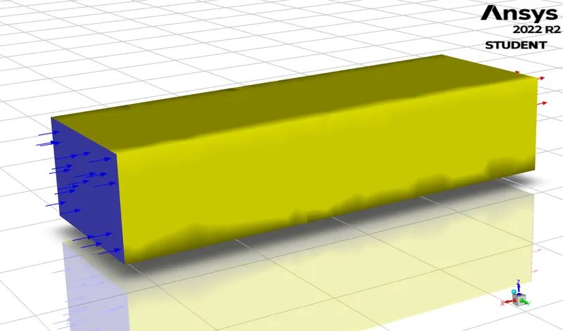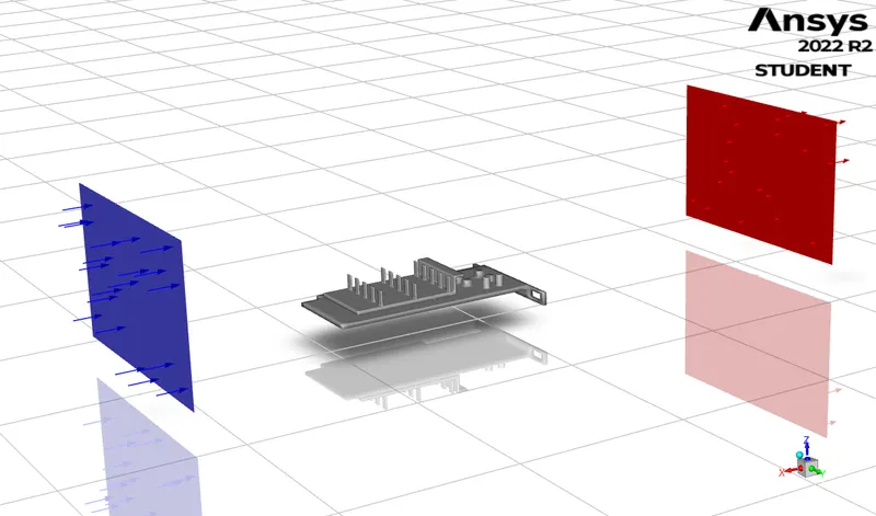
Graphic Card, Inlet, and Outlet in Fluent	Enclosure, Inlet, and Outlet in Fluent

iii. Steps to Set up the Physics: -

Fluent `->` Physics `->` Models `->` Viscous `->` `ubrace("Select Desired Viscous Model")_("In our case Select K-Omega SST")`

iv. Steps to Create desired Materials, Set Cells Zone and Set Heat Generation to Processor: -

a. Creating desired Materials: Fluent `->` Physics `->` Materials `->` Create/Edit... `->` `ubrace("Select/Create the desired Fluid")_("In our case, Create a Silicon and FR4")` `->` Enter

b. Setting Cell Zones: Fluent `->` Physics `->` Zones `->` Cell Zone `->` `ubrace("Select the desired Zone")_("In our case, Selected Fins, PCB and Processor")` `->` `ubrace("Set the Desired Type")_("Set Fins, PCB and Processor type to Solid")` `->` Edit `->` Set Desired Material for each Components `->` Apply

c. Setting Heat Generation to Processor: Fluent `->` Physics `->` Zones `->` Cell Zone `->` `ubrace("Select the desired Zone")_("In our case, Selected Processor")` `->` Edit `->` Select Source Term `->` Select "edit" from Energy under Source Term `->` Set Value to 1 `->` Added the Heat Generation Value `->` Ok `->` Apply

v. Steps to Set Boundary Conditions: -

Fluent `->` Physics `->` Zone `->` Boundaries `->` Select the desired Component `->` Select the Desired Type for that Component `->` Edit `->` Add the Values for the Component `->` Apply & Close

iv. Steps to Initialize and Set Desired Graphical Views: -

a. Initializing: Fluent `->` Solution `->` Initialization `->` Initialize

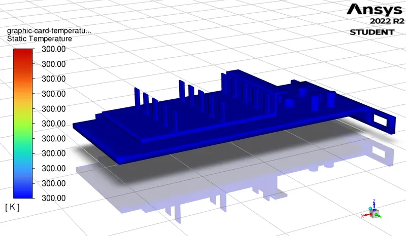
b. Setting the desired Contour: Fluent `->` Results `->` Graphics `->` Contours `->` New `->` Rename `->` Select Variable for Contour of `->` Select Surface `->` Save/Display

Steps to Analyse the Conjugate Heat Transfer Analysis of Exhaust Port: -

A. Performing Calculations and Developing Results: -

i. Steps to Open Fluent: -

Ansys Workbench `->` Project Schematic `->` Project `->` Setup `->` Right-Click `->` Edit

ii. Steps to Run Calculations: -

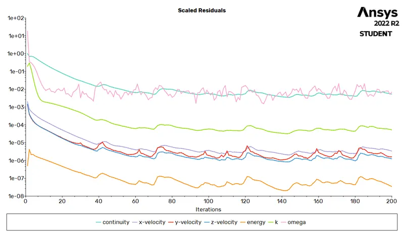
a. Setting No. of Iterations: Fluent `->` Solution `->` Run Calculations `->` `ubrace("Setting Desired Iterations in No. of Iterations")_("In Our Case, No. of Iterations is set to 200")`

b. Running Calculations: Fluent `->` Solution `->` Run Calculations `->` Calculate

Output/Results Generated after Analysis: -

A. For Inlet Velocity = 1 m/sec

i. Plots and Calculations: -

Residual Plot	Calculations Results
Average Fin Temperature Plot	Average Processor Temperature Plot

ii. Contours Generated: -

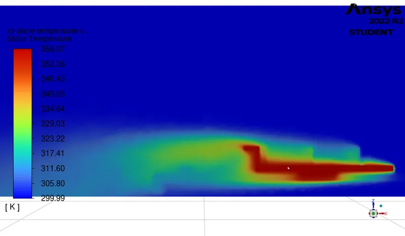Graphics Card Temperature Contour	XZ Plane Temperature Contour
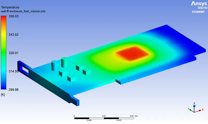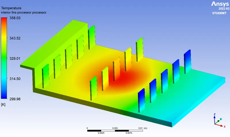
Fins Temperature Contour	PCB Temperature Contour
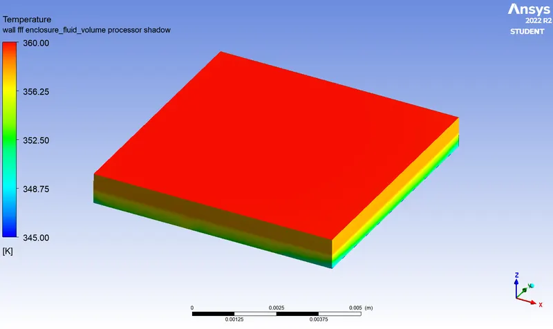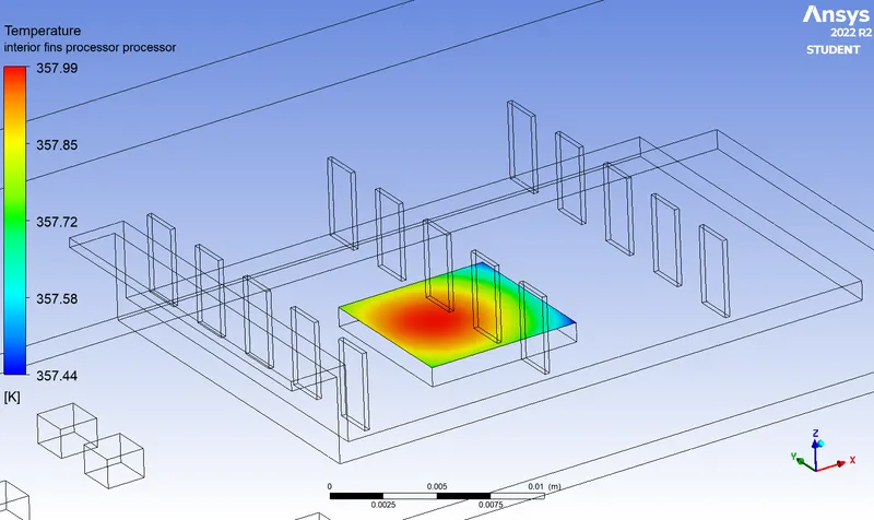
Top Processor Surface Temperature Contour	Processor Temperature Contour

B. For Inlet Velocity = 3 m/sec

i. Plots and Calculations: -

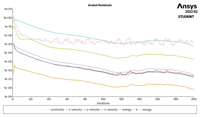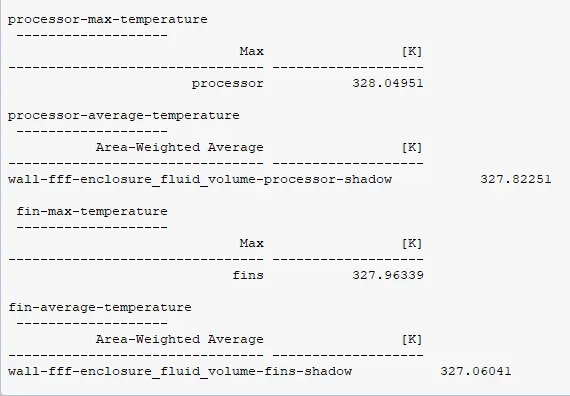Residual Plot	Calculations Results
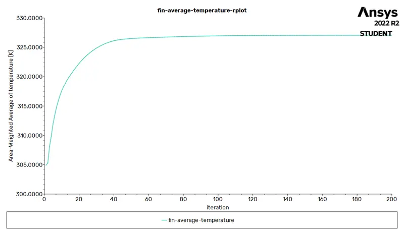Average Fin Temperature Plot	Average Processor Temperature Plot

ii. Contours Generated: -

Graphics Card Temperature Contour	XZ Plane Temperature Contour
Fins Temperature Contour	PCB Temperature Contour
Top Processor Surface Temperature Contour	Processor Temperature Contour

A. For Inlet Velocity = 5 m/sec

i. Plots and Calculations: -

Residual Plot	Calculations Results
Average Fin Temperature Plot	Average Processor Temperature Plot

ii. Contours Generated: -

Graphics Card Temperature Contour	XZ Plane Temperature Contour
Fins Temperature Contour	PCB Temperature Contour
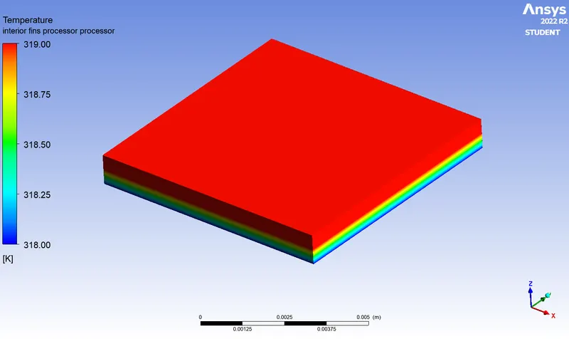Top Processor Surface Temperature Contour	Processor Temperature Contour

Observations and their Reasons: -

A. Benefits of the presence of Fins: -

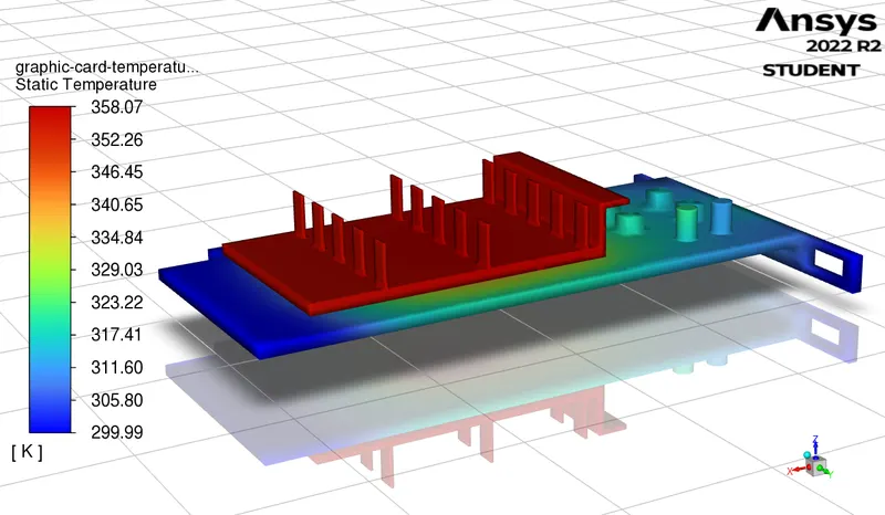
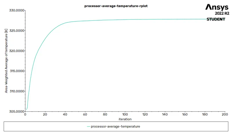
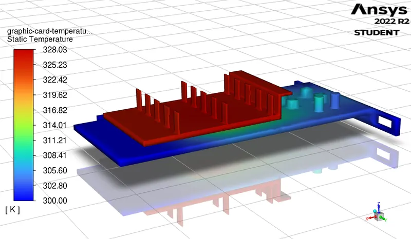
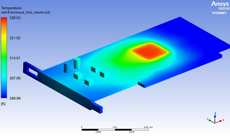
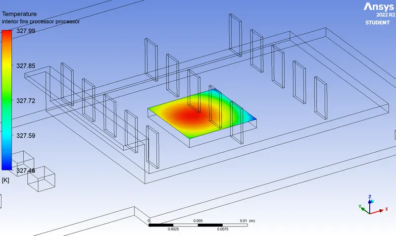
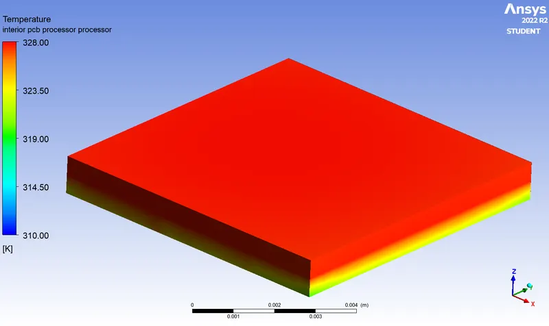
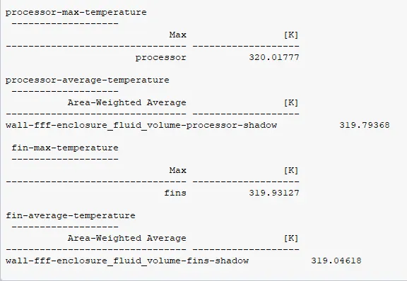
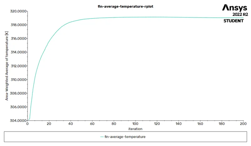
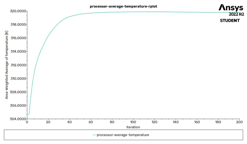
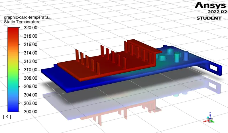
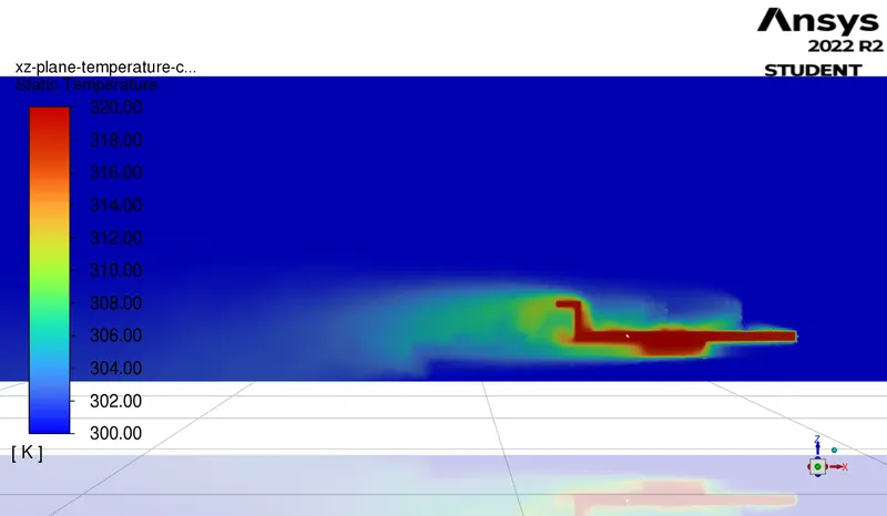
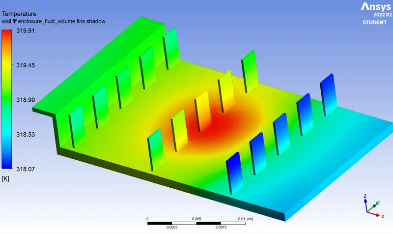
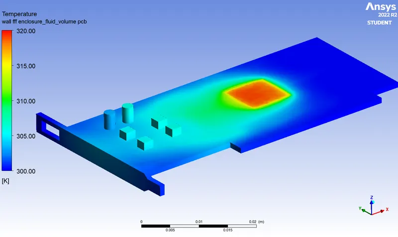
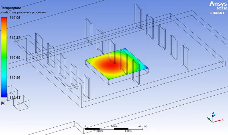
As can be observed for the given cases above the Temperature of the Processor and Fins are nearly the same this is because the material of the fins is copper. Due to the higher surface area due to the presence of the Fins, the Processor remains relatively cool and is effectively able to remove heat from the System.

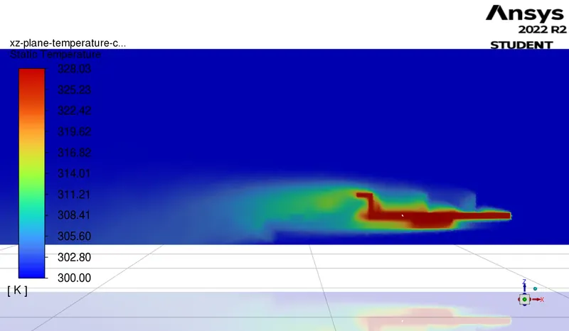
But it can be observed from the XZ Plane Temperature Contour that the flow of the Fluid is obstructed which reduces the net effectiveness of the Fins which can be improved if all the Fins are arranged in the XZ direction rather than the YZ direction.

B. Hot Spots: -

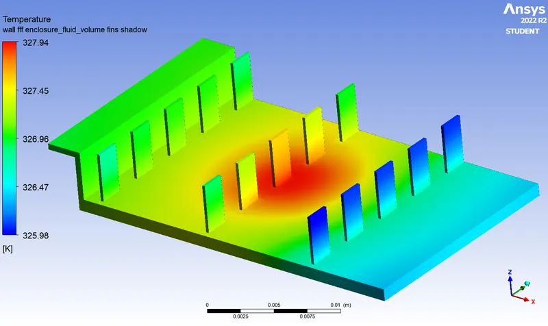
The Hot Spots of the system are the Zone on the Fin that is in contact with the fin, the following are ways to reduce the temperature of the Hot Spots: -

i. Increase the Number of Fins in the region.

ii. Arrange the Fins along the XZ direction to create an unobstructed flow of fluid which will improve the heat removal rate.

Click Here to Download the Ansys Files for this Challenge