Week 6 - CHT Analysis on a Graphics card

CHT ANALYSIS OF GRAPHICS CARD

1. OBJECTIVE

To simulate the CHT analysis of given graphics card under various boundary conditions, and to obtain the maximum temperature and heat transfer coefficient attained by the processor.

2. 3D MODEL

A simplified model of graphics card is used for the CHT analysis as complex designs lead to higher mesh metrics which cannot be run easily. The model consists of a fin, processor, and a base.

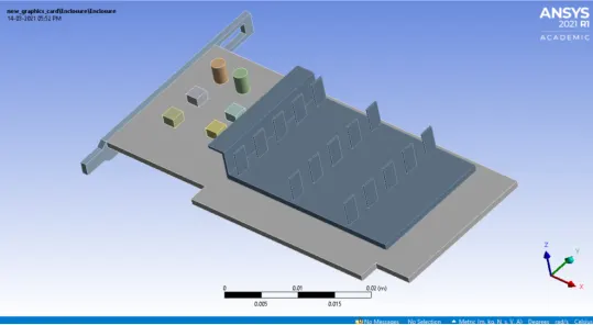
Fig.2.1: Graphics Card - Isometric View

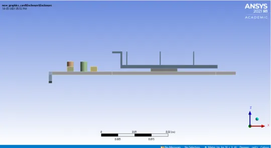
Fig. 2.2: Graphics Card - Side View

3. MESH DETAILS

Table 3.1: Refined Mesh Details

METRICS	VALUE
FIN	HEX DOMINANT - QUAD/TRI
PROCESSOR	MULTIZONE - HEXA MAPPED
BASE	HEX DOMINANT - QUAD/TRI
MESH SIZE (FIN)	1e-3 m
MESH SIZE (PROCESSOR)	1e-3 m
MESH SIZE (BASE)	1e-3 m
MESH SIZE (ENCLOSURE)	2.5e-3 m
ELEMENTS	413890
NODES	76482

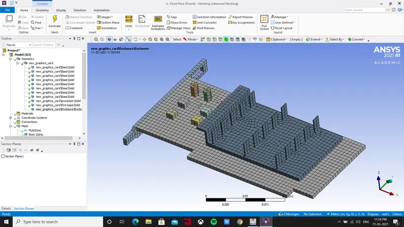
Fig. 3.1. Graphics Card (Isometric View)

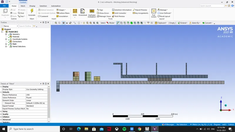
Fig.3.2. Graphics Card (Side View)

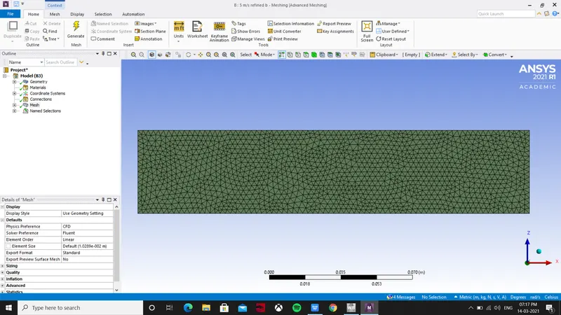
Fig.3.3. Fluid Volume

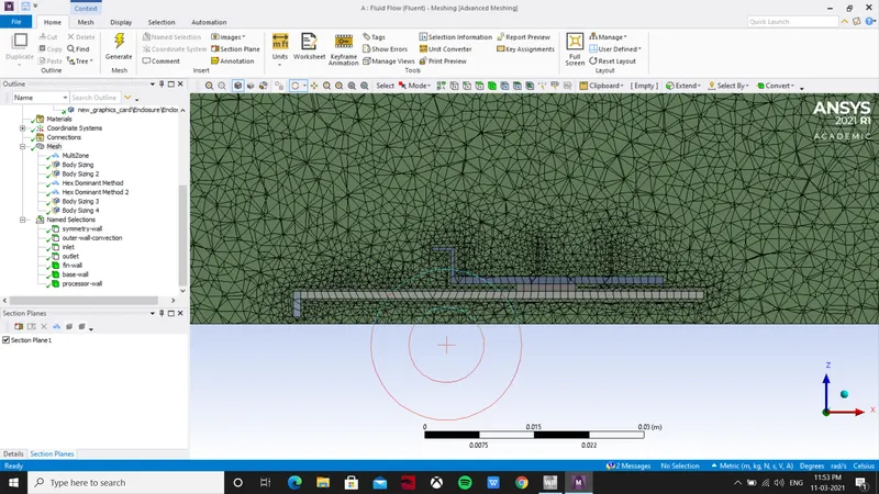
Fig. 3.4. Fluid Volume - Sectional View

4. MATERIAL PROPERTIES

Table 4.1: Material Property (Fin)

METRICS	VALUE
MATERIAL	ALUMINIUM
DENSITY	2719 kg/m3
SPECIFIC HEAT	871 J/kg-K
THERMAL CONDUCTIVITY	202.4 W/m-K

Table 4.2: Material Property (Processor)

METRICS	VALUE
MATERIAL	COPPER
DENSITY	8978 kg/m3
SPECIFIC HEAT	381 J/kg-K
THERMAL CONDUCTIVITY	387.6 W/m-K

Table 4.3: Material Property (Base)

METRICS	VALUE
MATERIAL	STEEL
DENSITY	8030 kg/m3
SPECIFIC HEAT	502.48 J/kg-K
THERMAL CONDUCTIVITY	16.27 W/m-K

Table 4.4: Material Property (Fluid Volume)

METRICS	VALUE
MATERIAL	AIR
DENSITY	1.225 kg/m3
SPECIFIC HEAT	1006.43 J/kg-K
THERMAL CONDUCTIVITY	0.0242 W/m-K
VISCOSITY	1.7894e-05 kg/m-s

5. BOUNDARY CONDITIONS

The inlet conditions were varied to determine the effect of velocity in heat transfer rate.

Table 5.1: Boundary Conditions

METRICS	VALUE
INLET	1, 3, 5 m/s
OUTLET (GAUGE PRESSURE)	0 Pa
HEAT FLUX (PROCESSOR)	2.7e5 W/m2

6. RESULTS

6.1. VELOCITY = 1 MPS

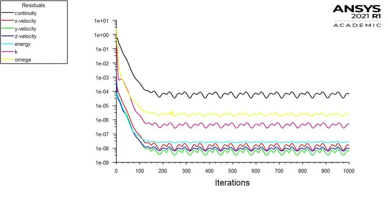
Fig.6.1.1. Residuals Report - 1 MPS

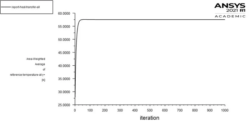
Fig.6.1.2. Heat Transfer Coefficient Report - 1 MPS

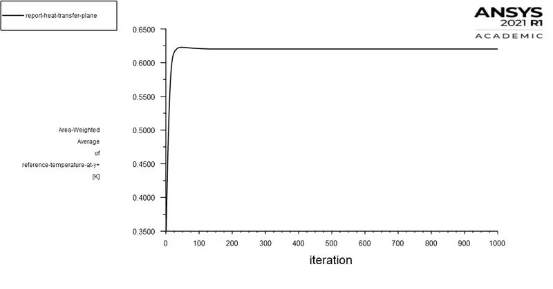
Fig.6.1.3. Heat Transfer Coefficient Report at Plane - 1 MPS

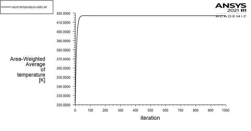
Fig.6.1.4. Static Temperature Report - 1 MPS

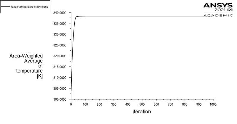
Fig.6.1.5. Static Temperature Report at Plane - 1 MPS

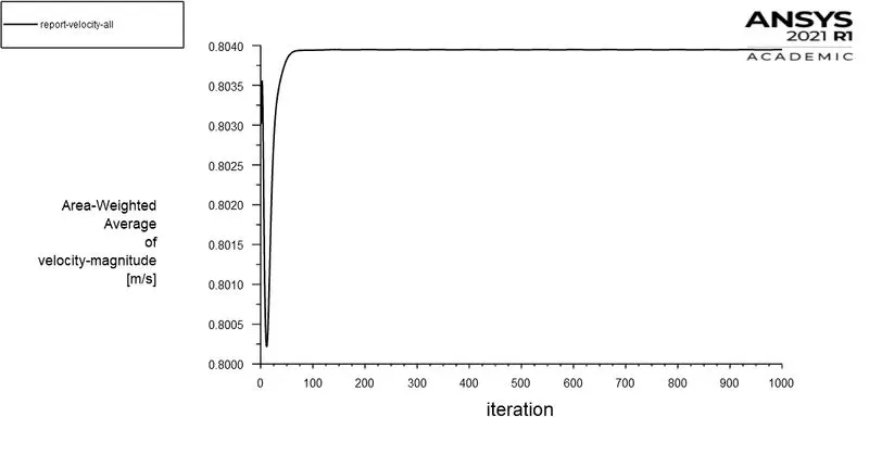
Fig.6.1.6. Velocity Report - 1 MPS

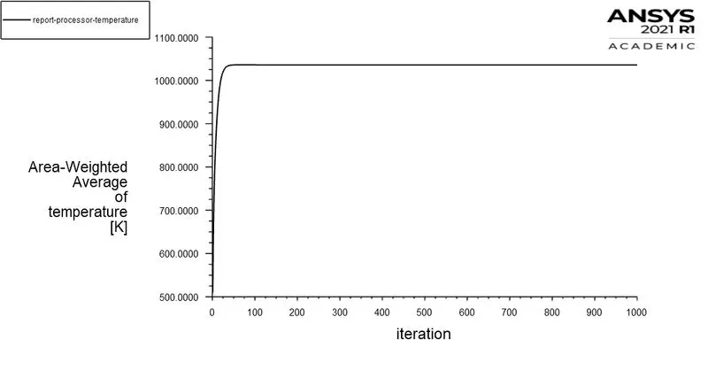
Fig.6.1.7. Processor Temperature - 1 MPS

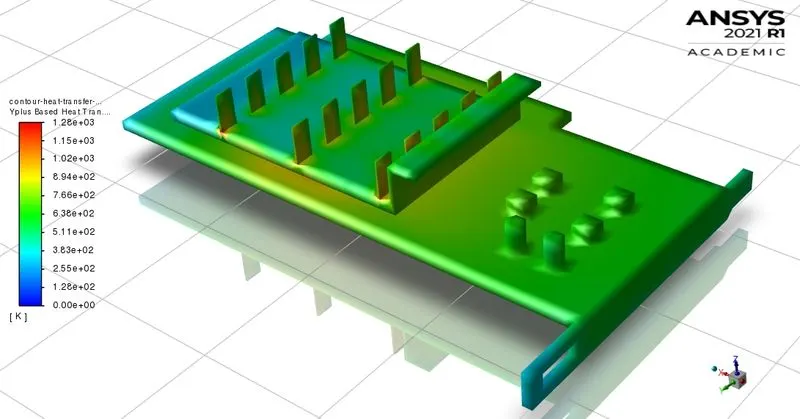
Fig.6.1.8. Isometric View of Heat Transfer Coefficient Contour - 1 MPS

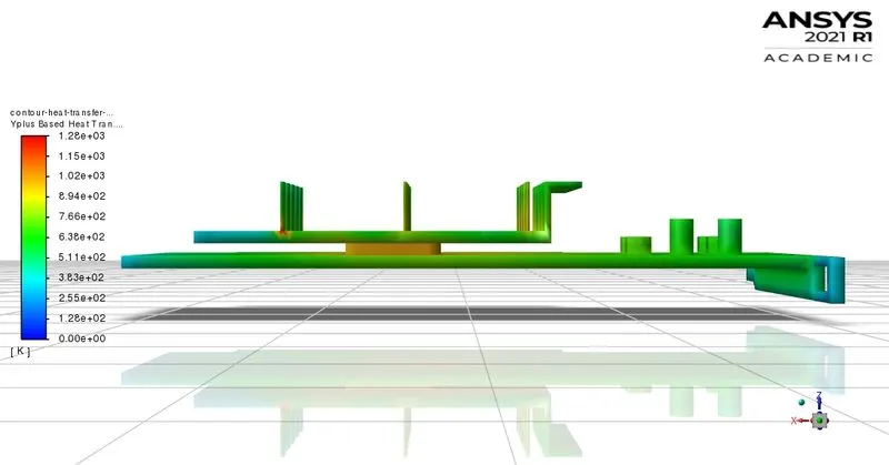
Fig.6.1.9. Side View of Heat Transfer Coefficient Contour - 1 MPS

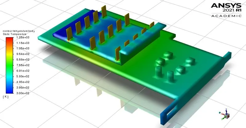
Fig.6.1.10. Isometric View of Temperature Contour - 1 MPS

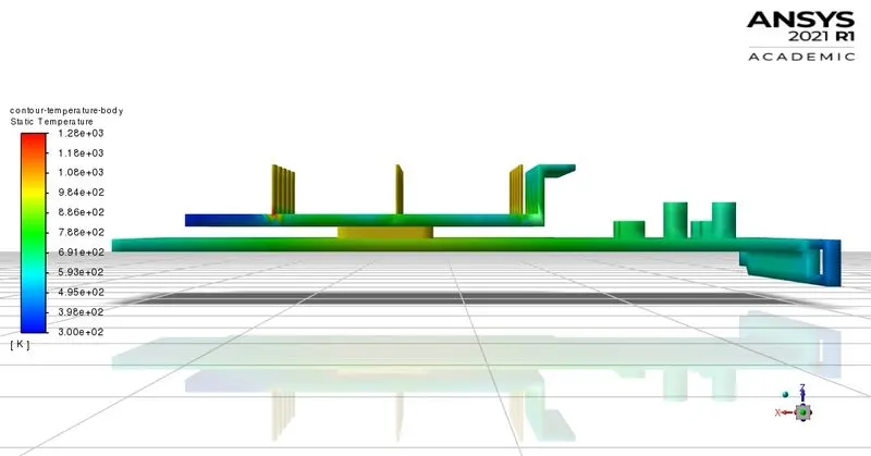
Fig.6.1.11. Side View of Temperature Contour - 1 MPS

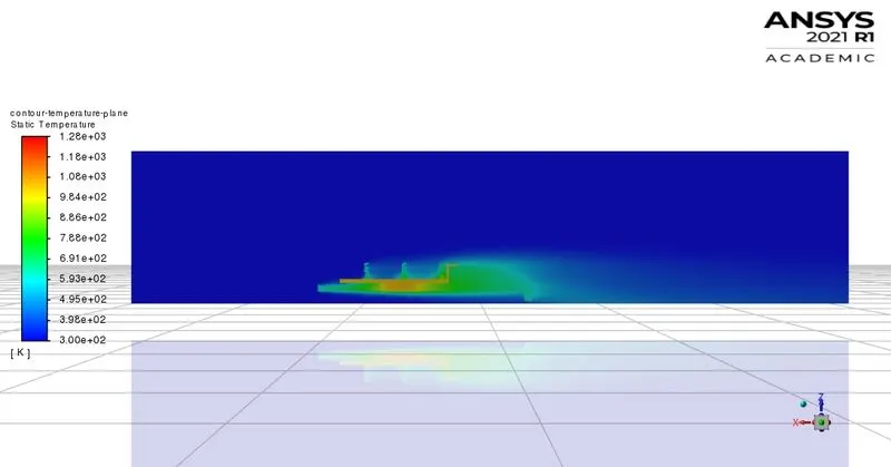
Fig.6.1.12. Temperature Contour at Plane - 1 MPS

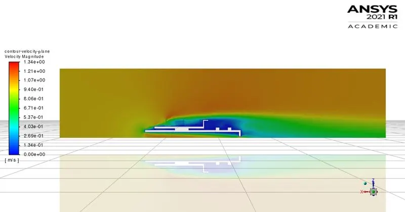
Fig. 6.1.13. Velocity Contour at Plane - 1 MPS

6.2. VELOCITY = 3 MPS

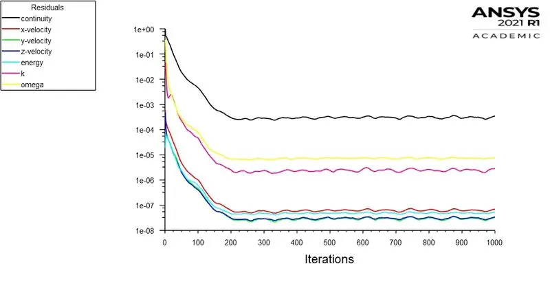
Fig.6.2.1. Residuals Report - 3 MPS

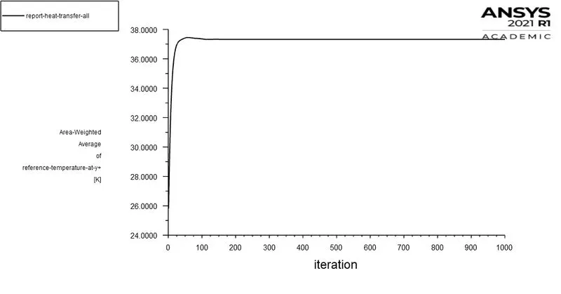
Fig.6.2.2. Heat Transfer Coefficient Report - 3 MPS

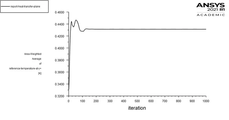
Fig.6.2.3. Heat Transfer Coefficient Report at Plane - 3 MPS

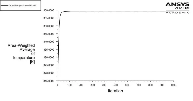
Fig.6.2.4. Static Temperature Report - 3 MPS

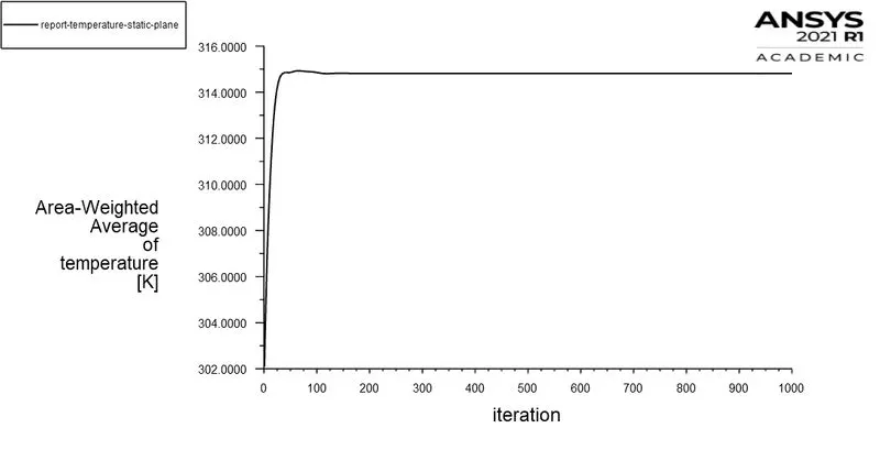
Fig.6.2.5. Static Temperature Report at Plane - 3 MPS

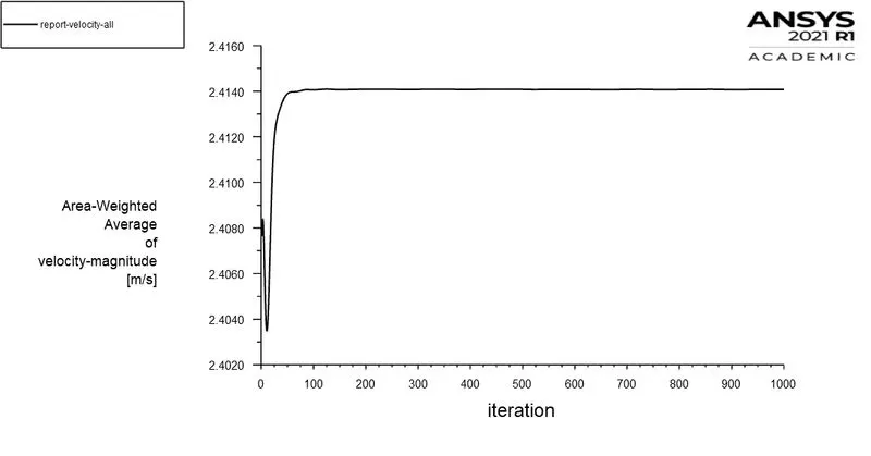
Fig.6.2.6. Velocity Report - 3 MPS

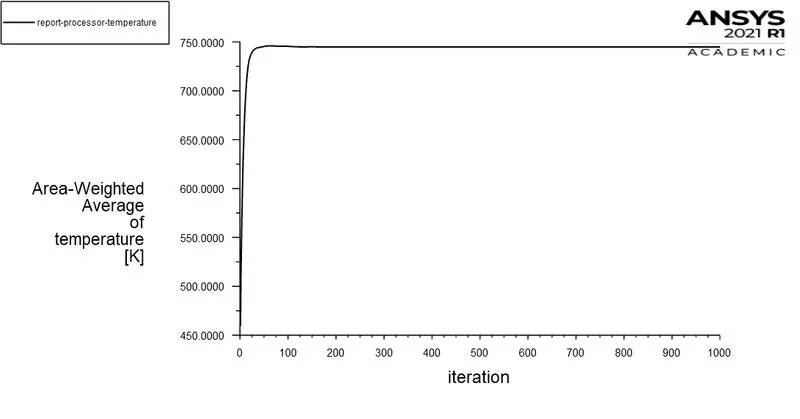
Fig.6.2.7. Processor Temperature - 3 MPS

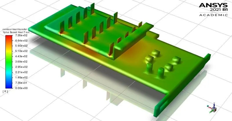
Fig.6.2.8. Isometric View of Heat Transfer Coefficient Contour - 3 MPS

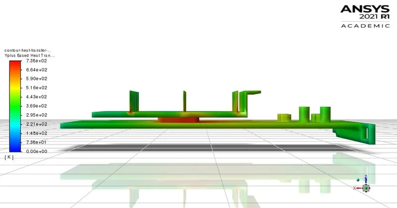
Fig.6.2.9. Side View of Heat Transfer Coefficient Contour - 3 MPS

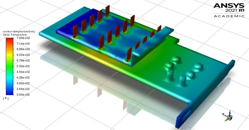
Fig.6.2.10. Isometric View of Temperature Contour - 3 MPS

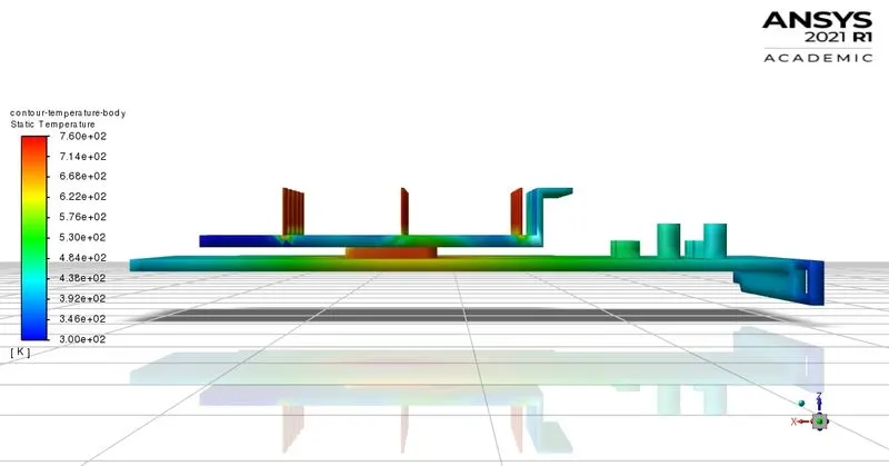
Fig.6.2.11. Side View of Temperature Contour - 3 MPS

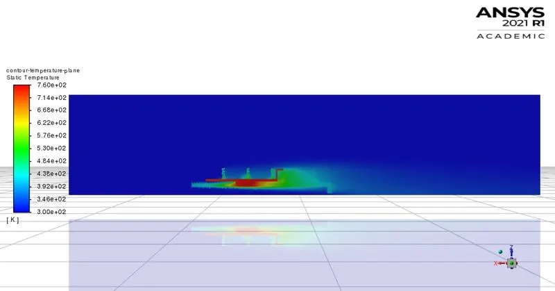
Fig.6.2.12. Temperature Contour at Plane - 3 MPS

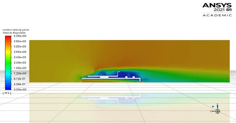
Fig. 6.2.13. Velocity Contour at Plane - 3 MPS

6.3. VELOCITY = 5 MPS

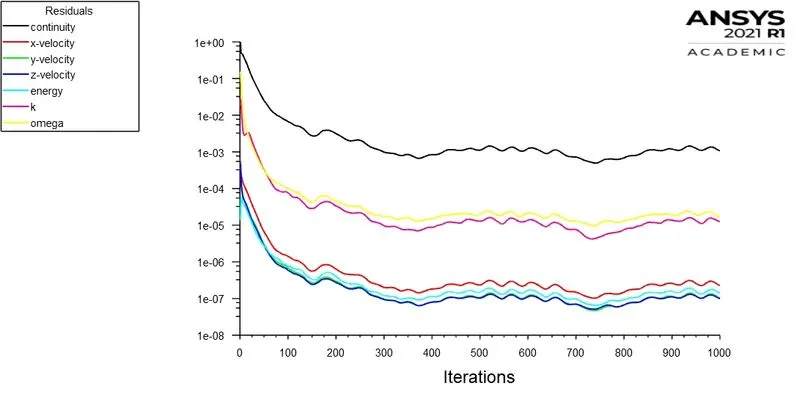
Fig.6.3.1. Residuals Report - 5 MPS

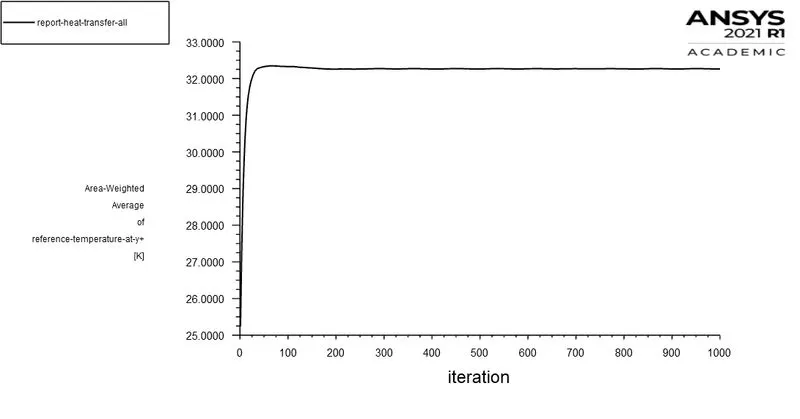
Fig.6.3.2. Heat Transfer Coefficient Report - 5 MPS

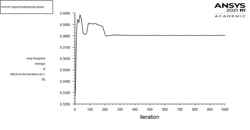
Fig.6.3.3. Heat Transfer Coefficient Report at Plane - 5 MPS

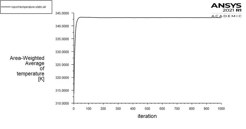
Fig.6.3.4. Static Temperature Report - 5 MPS

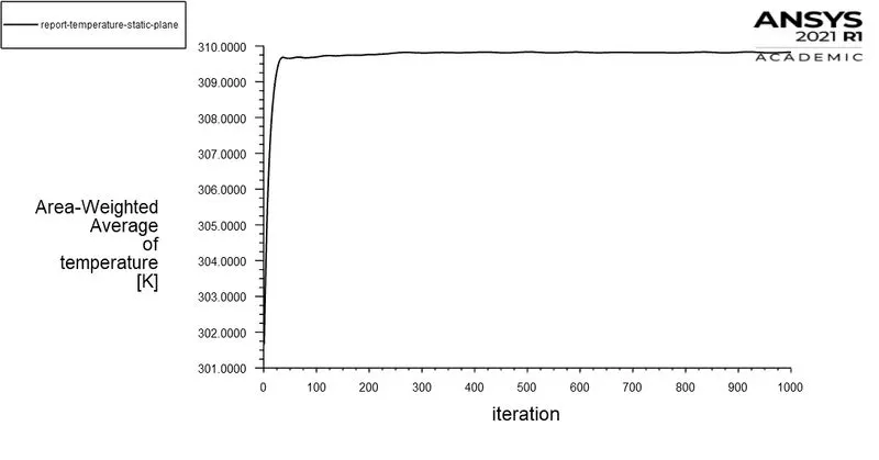
Fig.6.3.5. Static Temperature Report at Plane - 5 MPS

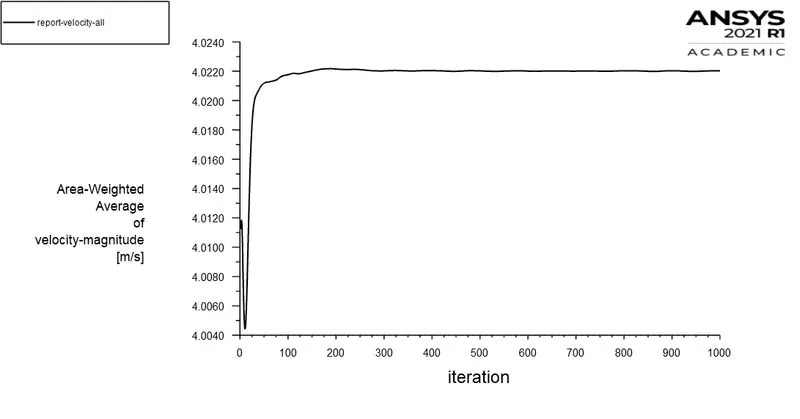
Fig.6.3.6. Velocity Report - 5 MPS

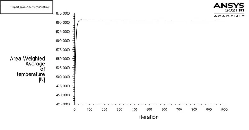
Fig.6.3.7. Processor Temperature - 5 MPS

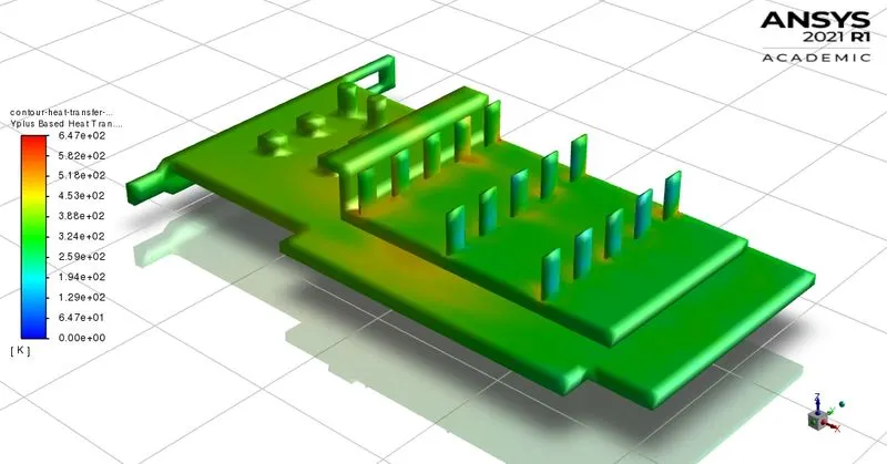
Fig.6.3.8. Isometric View of Heat Transfer Coefficient Contour - 5 MPS

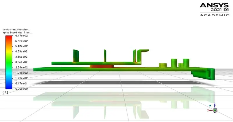
Fig.6.3.9. Side View of Heat Transfer Coefficient Contour - 5 MPS

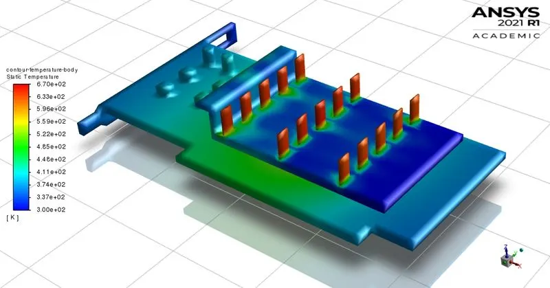
Fig.6.3.10. Isometric View of Temperature Contour - 5 MPS

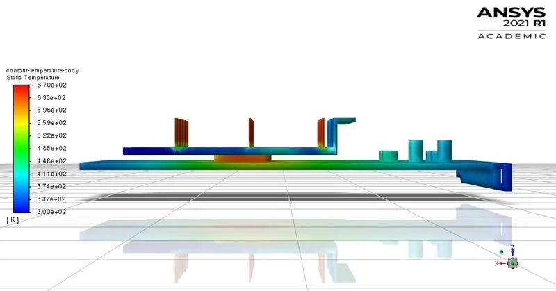
Fig.6.3.11. Side View of Temperature Contour - 5 MPS

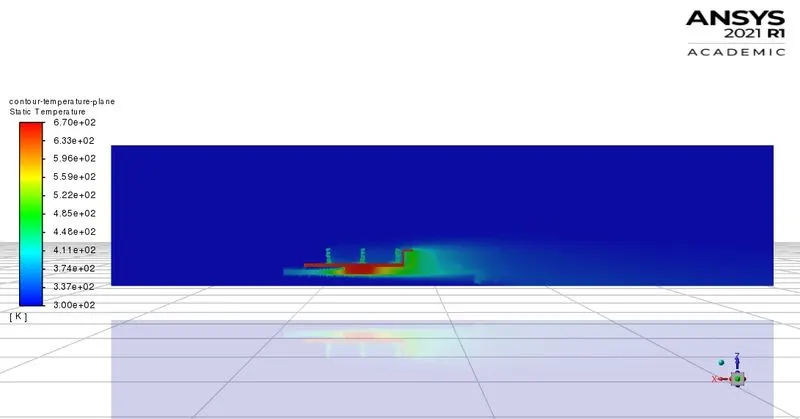
Fig.6.3.12. Temperature Contour at Plane - 5 MPS

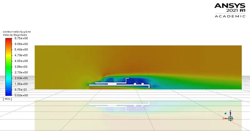
Fig.6.3.13. Velocity Contour at Plane - 5 MPS

7. CONCLUSION

• Convergence is achieved when the inlet velocity is increased.
• As the velocity increases, temperature around and behind the fin increases and decreases respectively due to low heat transfer around the fins.
• The processor attains highest temperature (1025 K) and Y-plus based Heat Transfer (8.94e+2) when velocity is 1 MPS.
• Fine mesh was utilized on fin and processor as heat transfer occurs primary around them, while coarse mesh was used on the base.
• Y-plus based heat transfer rate around the processor decreases when it is subjected to increasing velocity, resulting in effective cooling of processor.
• Primary hot-spots of temperature are around the processor on the base due to low heat transfer. As the velocity increases, the fins gets heated up due to low heat transfer with the fluid volume.