Mixing efficiency
Mixing Tee – Report
1. Objective
To simulate the mixing of two fluids (air) at different temperatures in a mixing tee and to determine the average temperature and its standard deviation at the outlet using two models in Ansys Fluent.
2. 3D Model
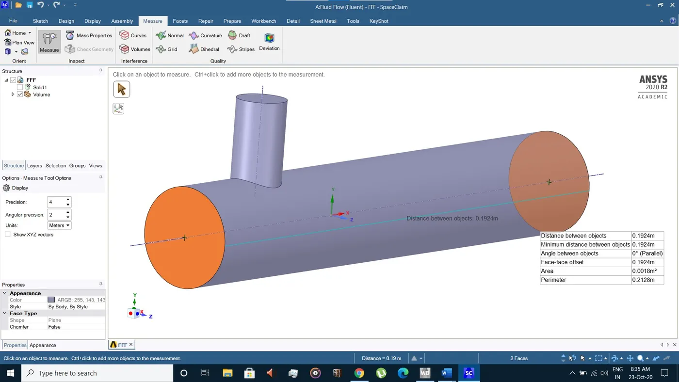
The 3D model comprises of a mixing tee having short and long dimensions at the throat to determine the effect of pipe length on mixing efficiency. Both the models are provided in the course, from which the fluid-volume is extracted and used for this project.
Length of short pipe (x-axis) = 0.1924 m
Length of long pipe (x-axis) = 0.2683 m
 |
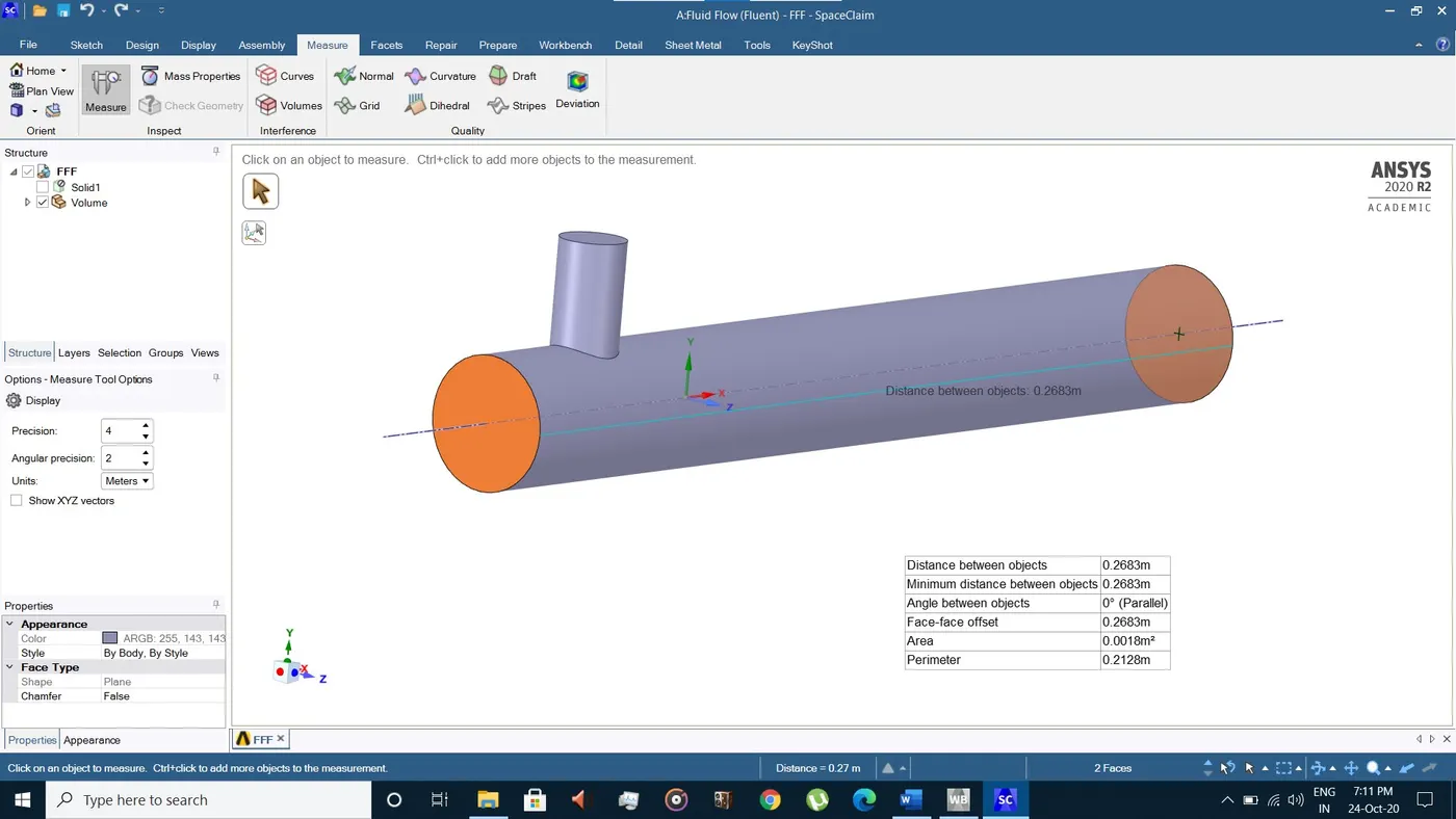 |
| Fig.1.1. Short Pipe – 3D Model | Fig.1.2. Long Pipe – 3D Model |
3. Mesh Details
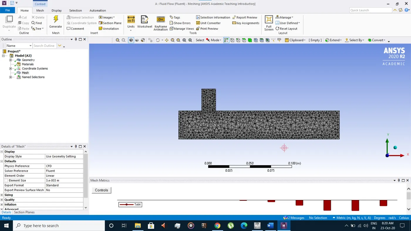
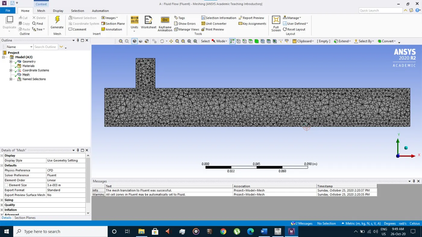
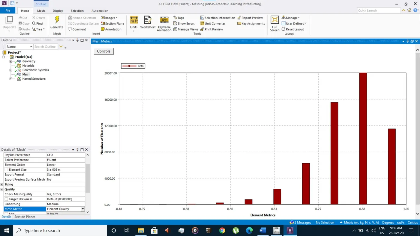
For both the pipes, three different mesh sizes had been used to determine the efficiency and accuracy of mixing of two fluids at different temperatures.
Table 1: Mesh Details
|
Pipe |
Mesh Size (m) |
Nodes |
Elements (Tetrahedral) |
|
Short |
0.004 |
4794 |
22284 |
|
0.003 |
8350 |
39817 |
|
|
0.0025 |
21330 |
105858 |
|
|
Long |
0.004 |
6252 |
29061 |
|
0.003 |
11689 |
56373 |
|
|
0.0025 |
28282 |
140025 |
 |
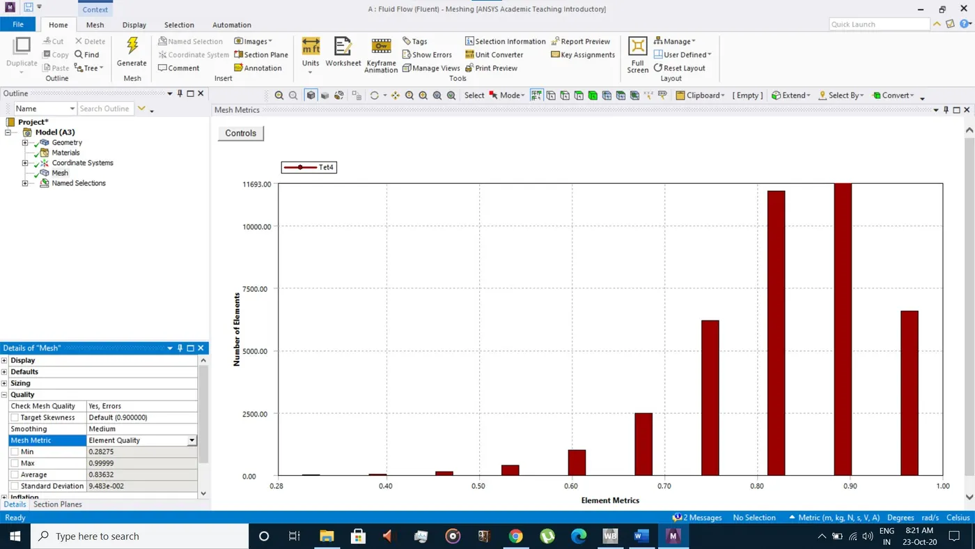 |
| Fig.2.1.1. Mesh of Short Pipe (Mesh size 0.003) | Fig.2.1.2. Mesh Chart of Short Pipe (Mesh size 0.003) |
 |
 |
| Fig.2.2.1. Mesh of Long Pipe (Mesh size 0.003) | Fig.2.2.2. Mesh Chart of Long Pipe (Mesh size 0.003) |
4. Material Properties
The fluid used in the mixing tee is air at different temperatures. The properties are briefed below.
Material/Material Type = Air/Fluid
Density = 1.225 kg/m3
Specific Heat (Cp) = 1006.43 J/kg-K
Thermal Conductivity (k) = 0.0242 W/m-K
Viscosity = 1.7894e-05 kg/m-s
5. Boundary Conditions
The initial boundary conditions are detailed below.
Hot air temperature = 36°C
Cold air temperature = 19°C
Velocity of hot air = 3 m/s
Momentum ratio = 2, 4
From calculations, the velocity of cold air are 6 m/s and 12 m/s respectively.
Planes at distances 0 m, 0.03 m, 0.06 m, and 0.09 m are created along the pipe for obtaining contours of temperature and velocity.
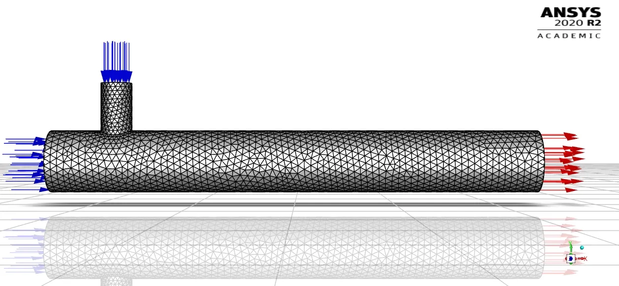 |
| Fig.3.1. Inlet and Outlet of Long Pipe |
6. Tabulations
CFD is done for both the pipes using K-Epsilon realizable and K-Omega SST model equations respectively. At the outlet, area-weighted reports of both average temperature and standard deviation of temperature is specified to check the outlet temperature. Initialization is done for 1000 iterations while the calculation of the residuals, standard deviation and average temperature is done till convergence all residuals is obtained. If not obtained, the calculation is done until 1000 iterations.
Table 2: Short Pipe
|
RANS Model Equation |
Cold Air Inlet Velocity (m/s) |
Cell Count |
Average Outlet Temperature (°C) |
Standard Deviation of Temperature (°C) |
No of Iterations for Convergence |
|
K - Epsilon |
6 |
22284 |
30.25 |
1.6 |
1000 |
|
39817 |
30.25 |
1.75 |
1000 |
||
|
105858 |
30.35 |
1.6 |
1000 |
||
|
12 |
22284 |
27.5 |
1.07 |
147 |
|
|
39817 |
27.6 |
1.08 |
178 |
||
|
105858 |
27.6 |
1.48 |
338 |
||
|
K - Omega |
6 |
22284 |
30.3 |
2.1 |
250 |
|
39817 |
30.35 |
2.3 |
270 |
||
|
105858 |
30.45 |
2.4 |
332 |
||
|
12 |
22284 |
27.6 |
1.38 |
188 |
|
|
39817 |
27.7 |
1.3 |
227 |
||
|
105858 |
27.7 |
2.2 |
1000 |
The results form CFD-post for the short pipe for both velocities clearly highlights the usage of both model equations, K-Epsilon in providing the efficiency of mixing at the middle of the pipe while K-Omega providing the same along with the mixing at the wall boundary.
As the number of iterations required for convergence is quite high and low for short pipe using K-Epsilon realizable model for both cold air inlet velocities respectively, the K-Omega model equation is used for the long pipe for both cold air inlet velocities. This is due to include of understanding the efficiency of mixing at the wall boundary. Also, the number of iterations for convergence using K-Omega SST model is quite low when compared to K-Epsilon realizable model.
The mesh size of 0.004 and 0.003 are quite satisfactory for the short mixing tee. The usage of 0.002 mesh size is to determine the exact boundary regions of temperature difference during mixing.
Table 3: Long Pipe
|
RANS Model Equation |
Cold Air Inlet Velocity (m/s) |
Cell Count |
Average Outlet Temperature (°C) |
Standard Deviation of Temperature (°C) |
No of Iterations for Convergence |
|
K - Omega |
6 |
29061 |
30.4 |
1.38 |
418 |
|
56373 |
30.45 |
1.85 |
250 |
||
|
140025 |
30.55 |
1.8 |
157 |
||
|
12 |
29061 |
27.5 |
0.86 |
152 |
|
|
56373 |
27.5 |
0.5 |
1000 |
||
|
140025 |
27.5 |
1.5 |
1000 |
Result
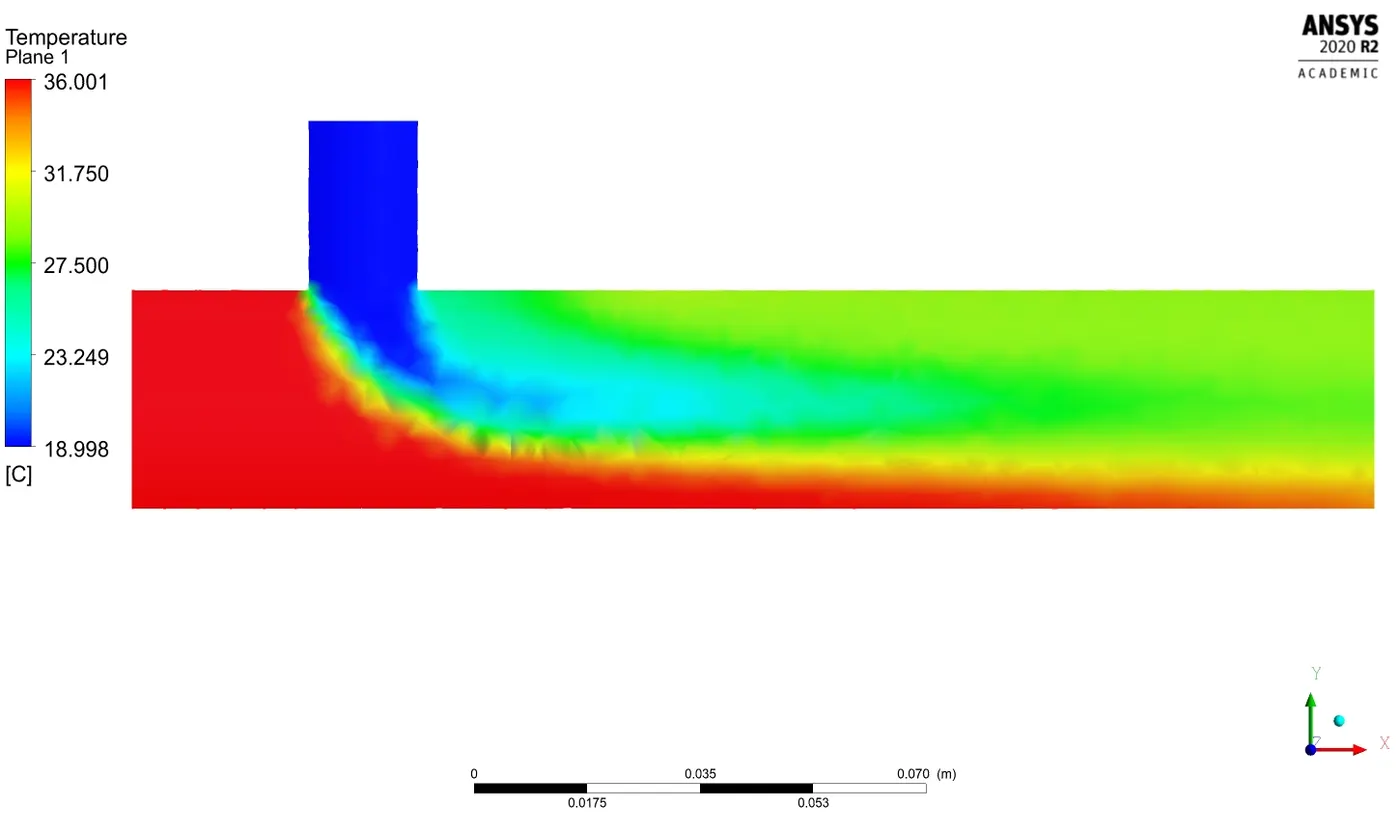
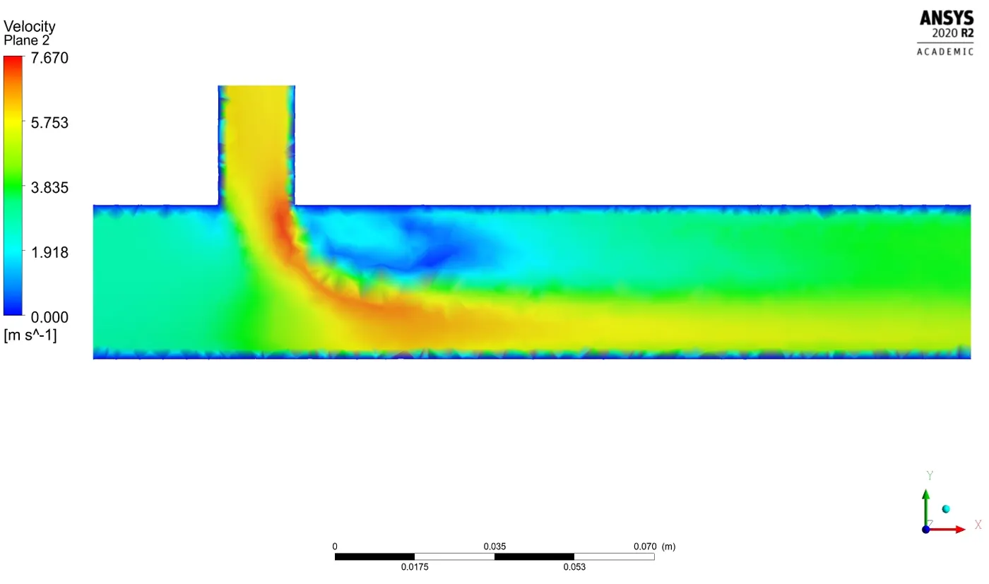
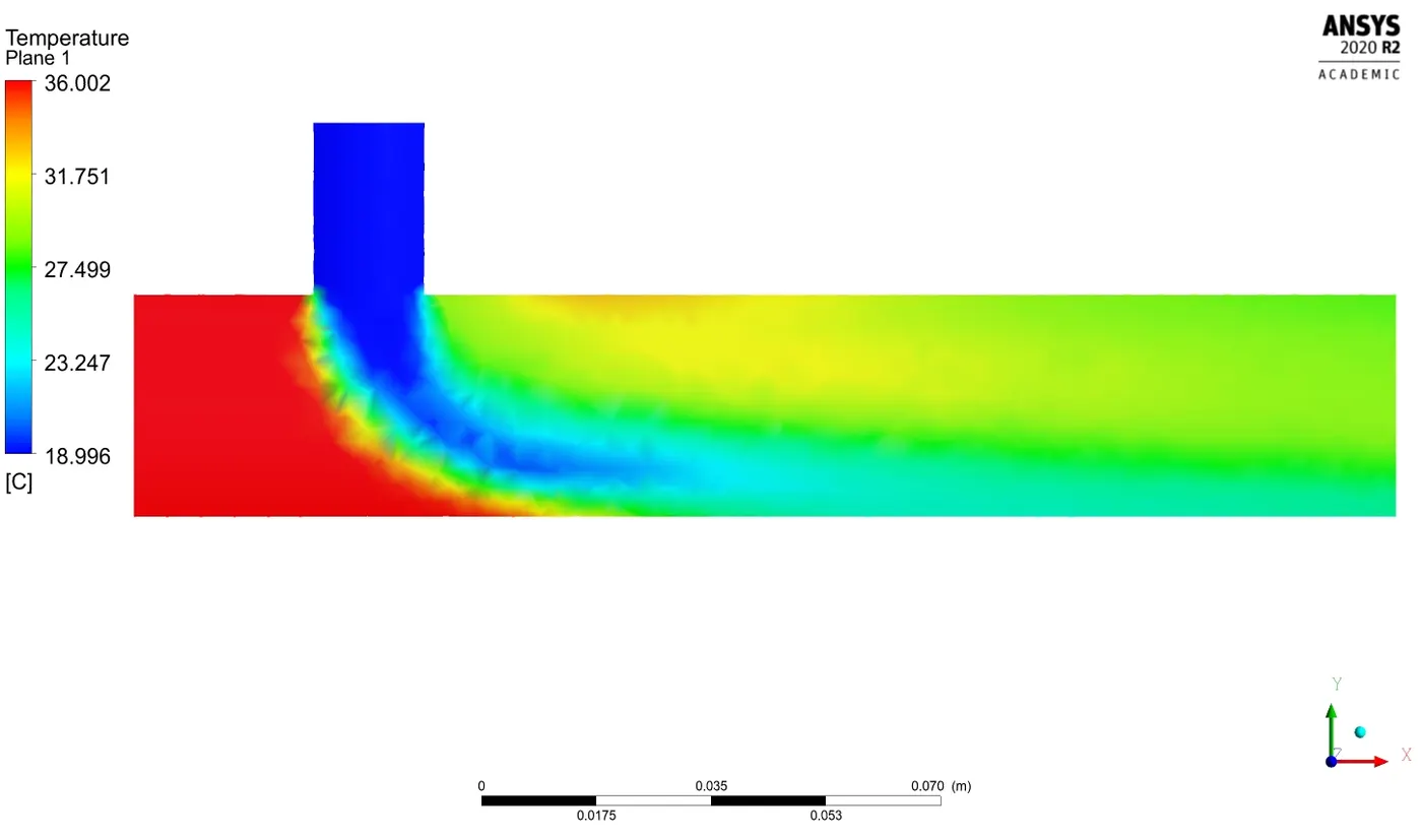
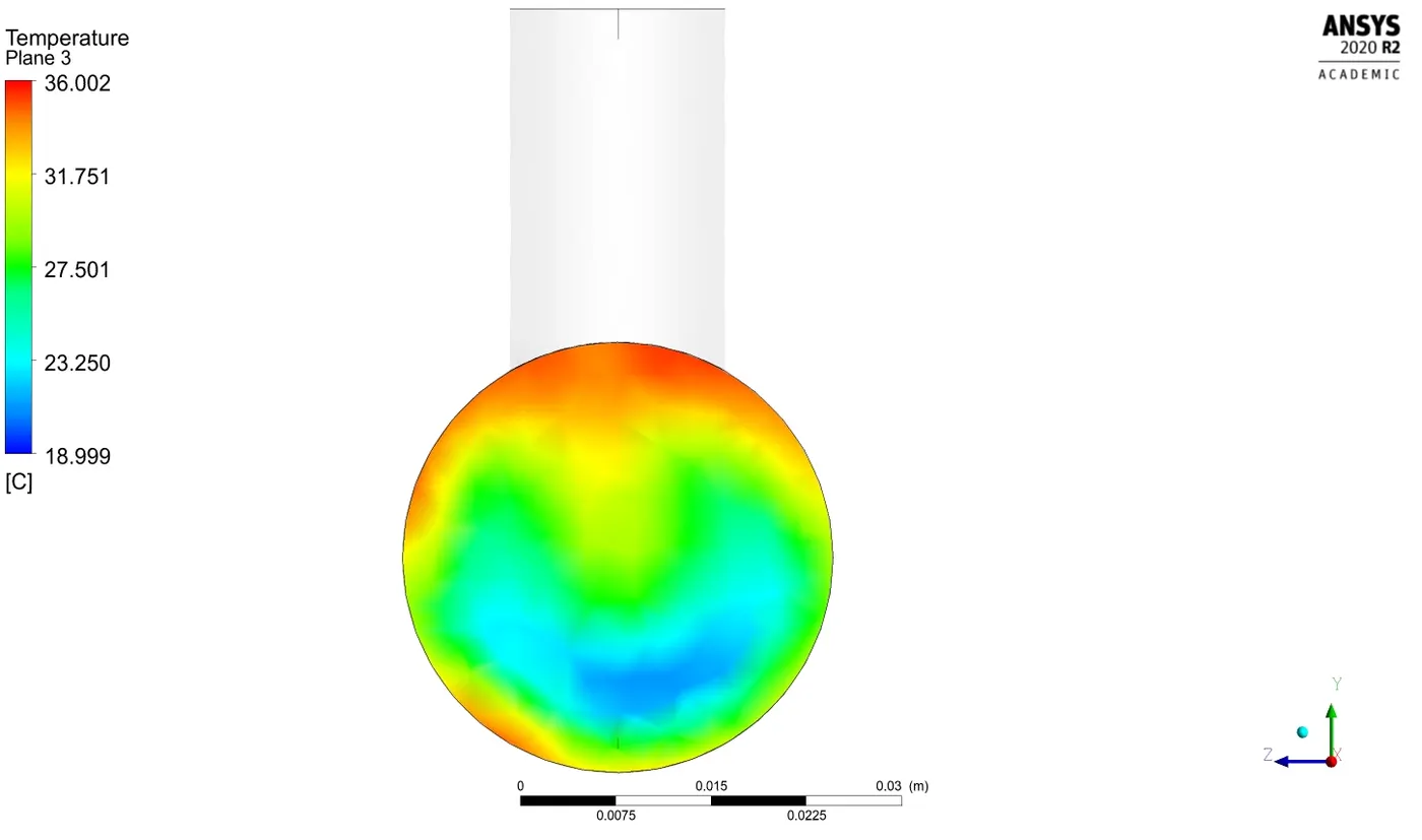
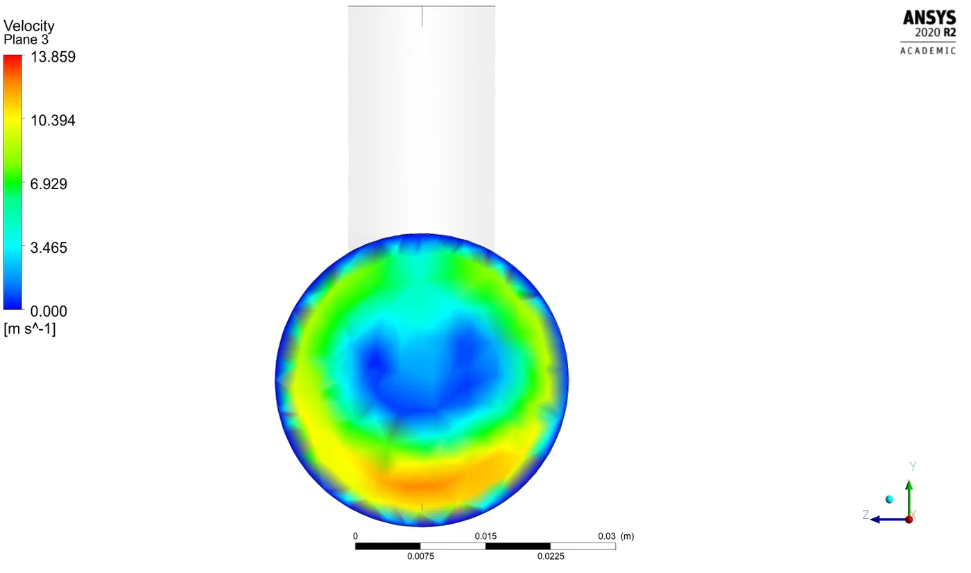
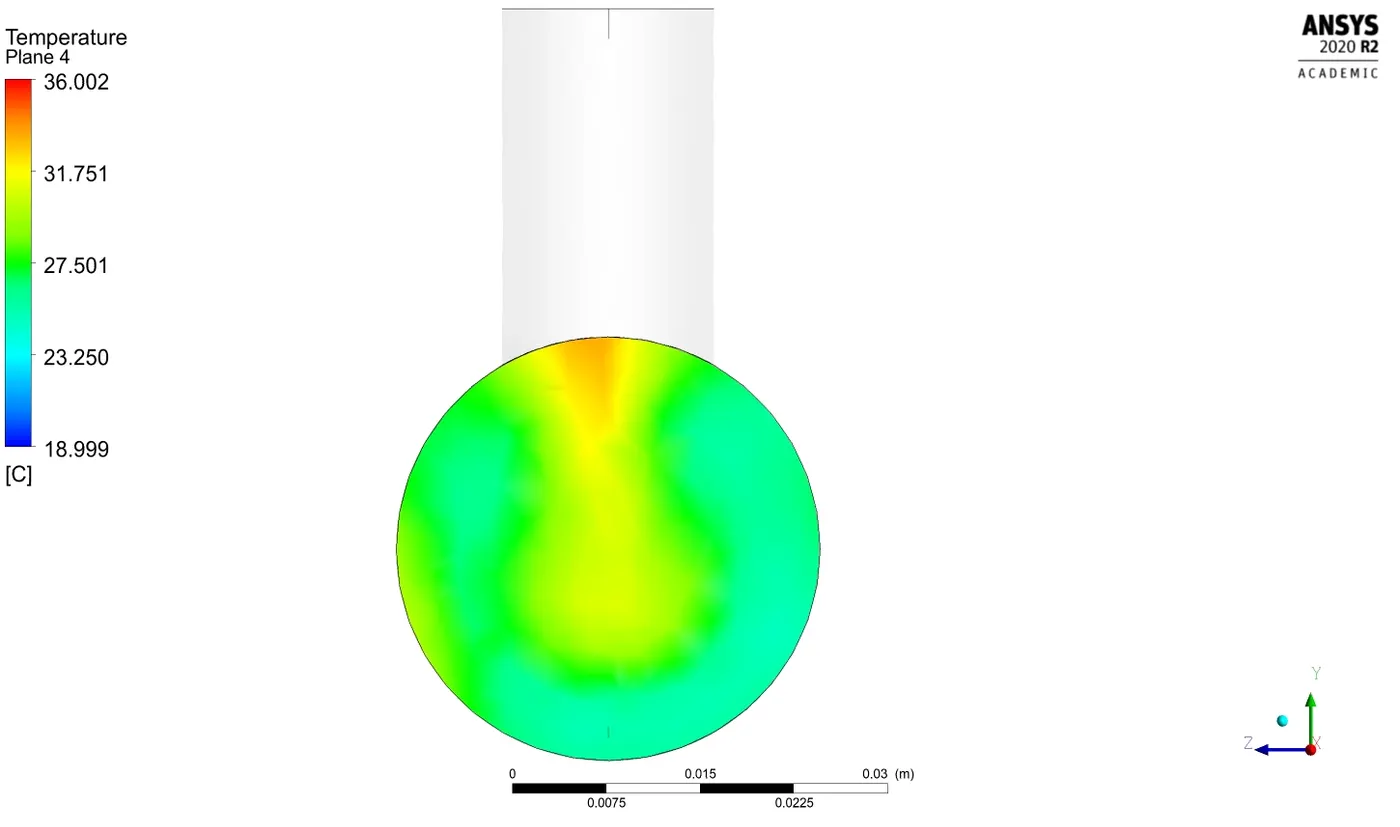
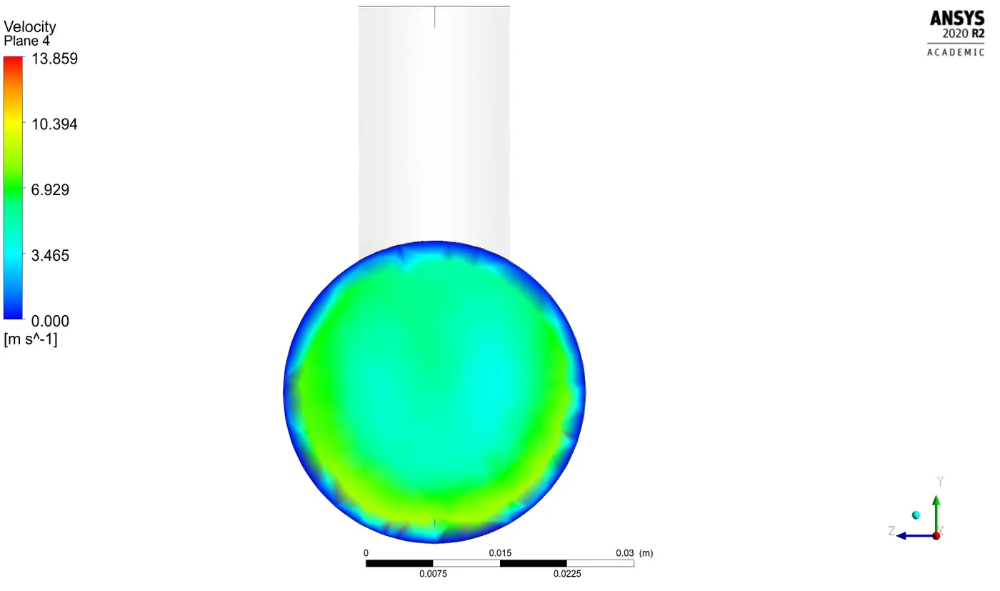
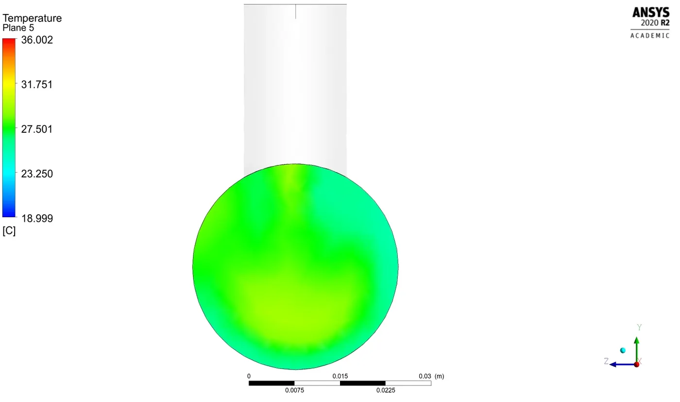
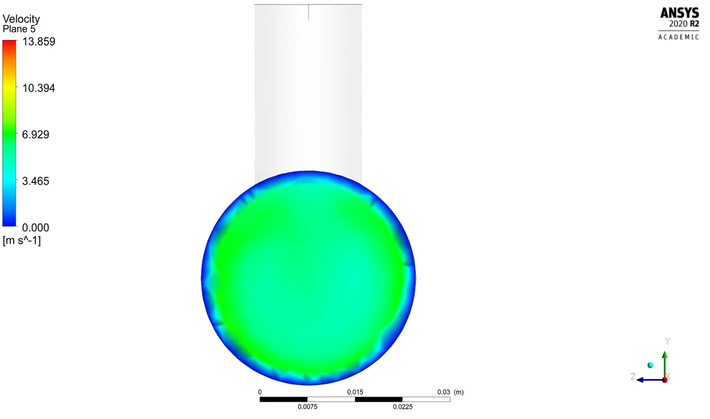
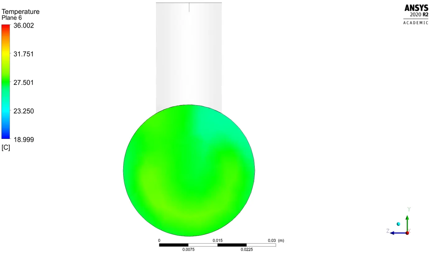
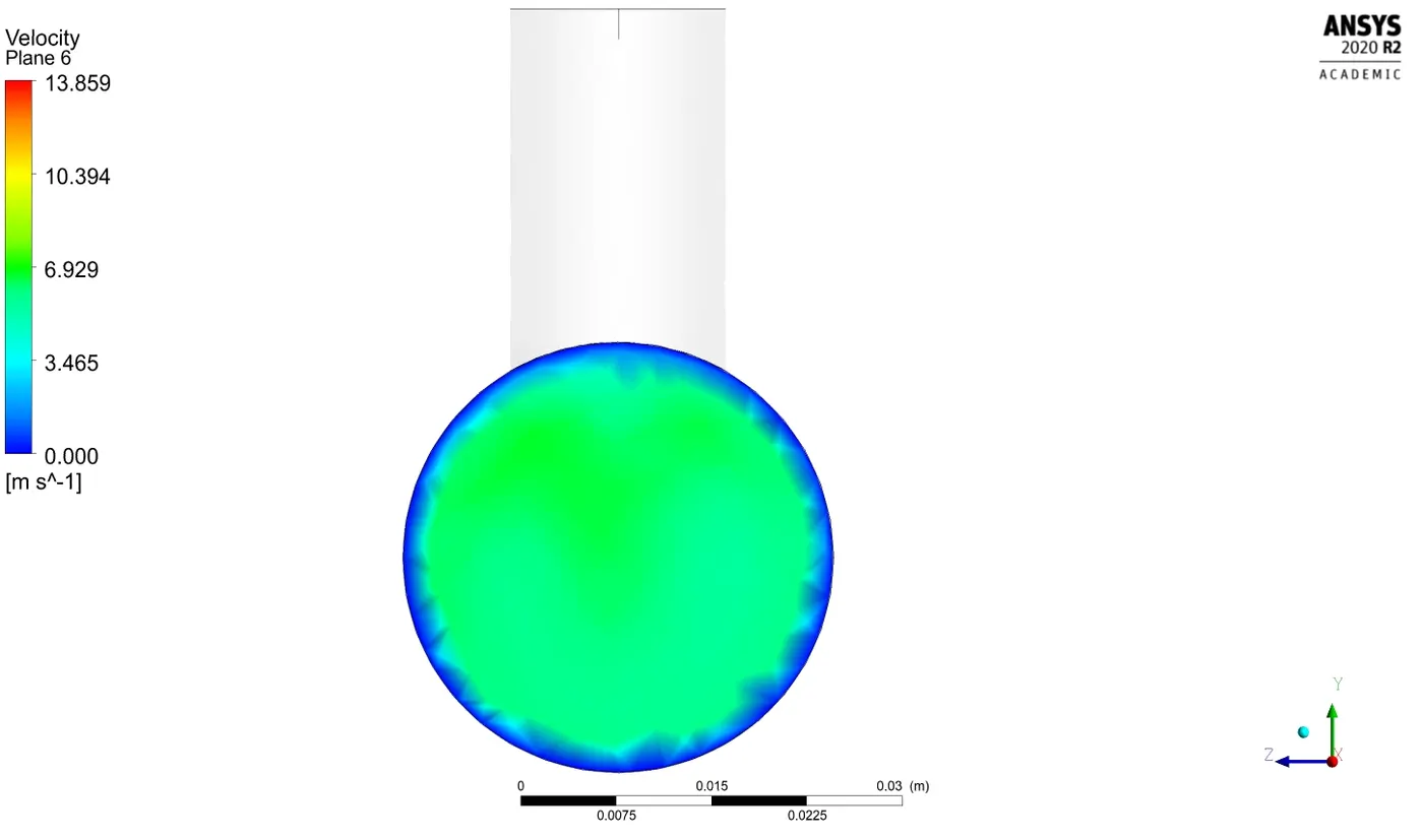
At the outlet, the temperature contours depict that the bottom of the pipe remains under the influence of hot air in the short and long pipe when an inlet of momentum ratio 2 is introduced. When the same pipe undergoes a momentum ratio of 4, the entire hot air is cooled after some distance along the cross-section. Also, a uniform cross-sectional temperature is obtained at the outlet. Moreover, a region of high temperature is obtained at the top boundary after the vertical inlet depicting some turbulence as the fluids mix. The velocity contours show negligible difference between both viscous model equations. As shown in temperature contours, the velocity contours display a region of turbulence at a position after the immediate mixing of two fluids.
| Momentum | Parameters | Short Pipe (K-Ω) | Short Pipe (K-ε) |
| Low | Temperature | 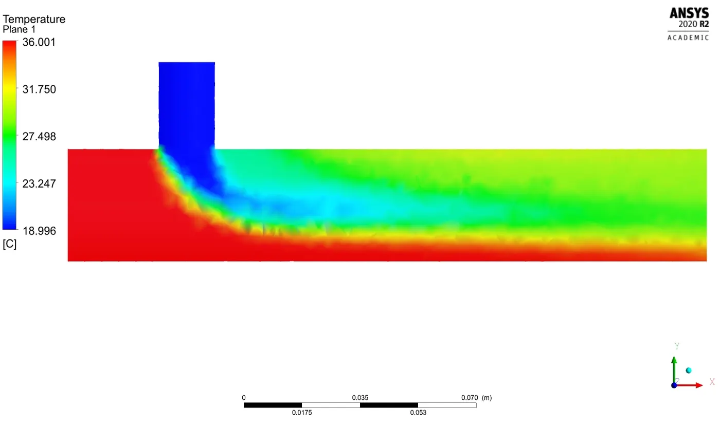 |
 |
| Velocity | 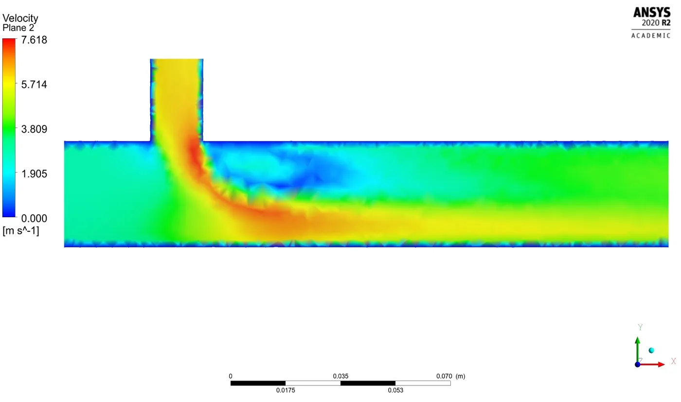 |
 |
|
| High | Temperature | 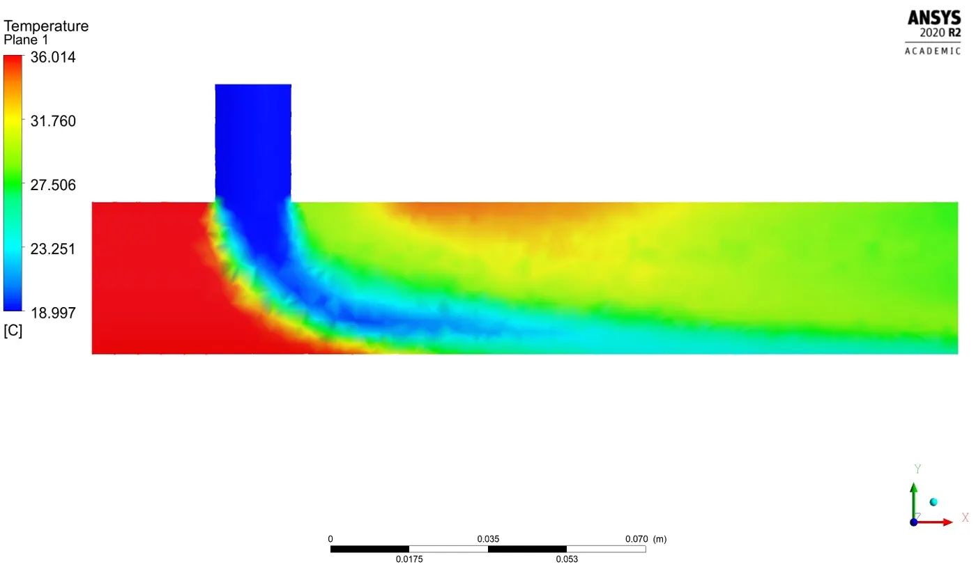 |
 |
| Velocity | 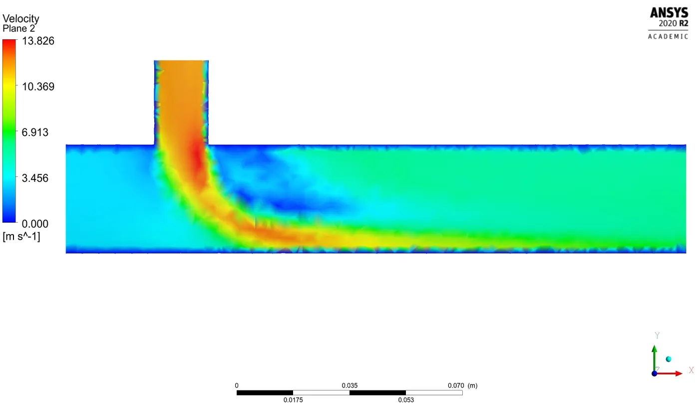 |
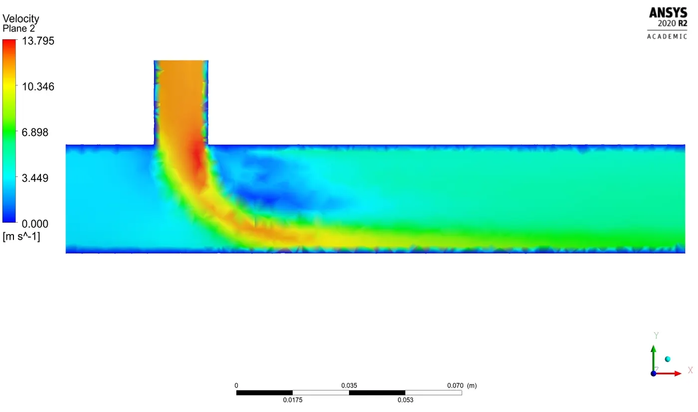 |
Fig.4.1. Short Pipe Length-Wise Temperature and Velocity Contours
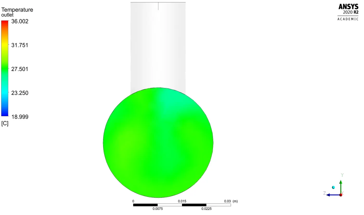
To determine the effect of change in momentum on the long pipe, planes were placed at four different locations (0.15m, 0.2m, 0.25m, 0.3m, 0.35m) from the inlet at x-axis. The temperature and velocity contours were traced and analyzed. The contours showed that the higher momentum produced quicker mixing of the fluids and a laminar flow of around 5m/s at the outlet.
| Length (m) | Parameter | Low Inlet Momentum | High Inlet Momentum |
| 0.15 | Temperature | 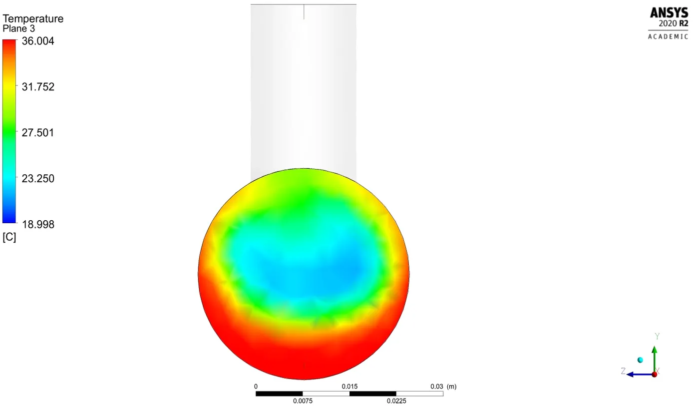 |
 |
| Velocity | 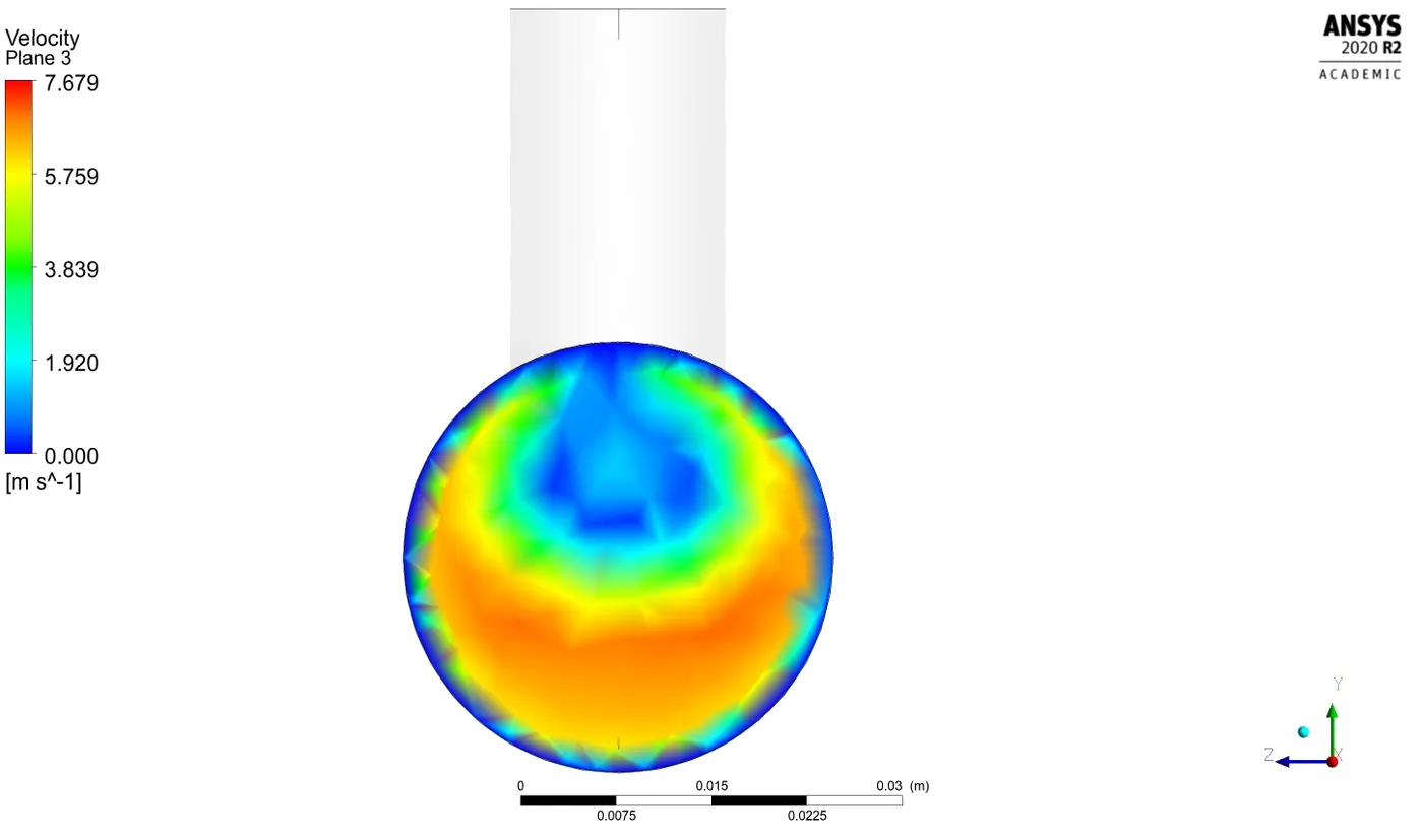 |
 |
|
| 0.2 | Temperature | 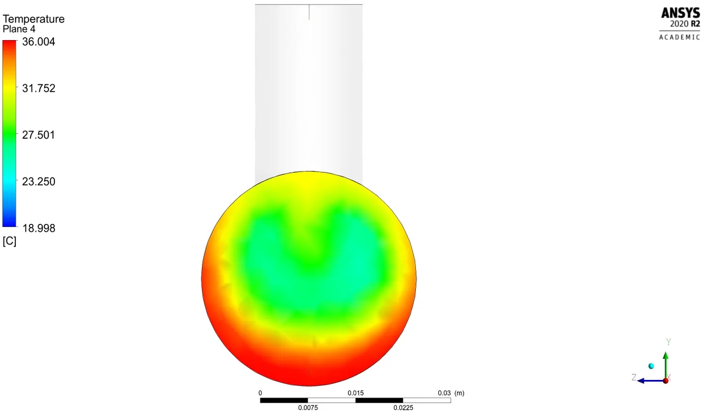 |
 |
| Velocity | 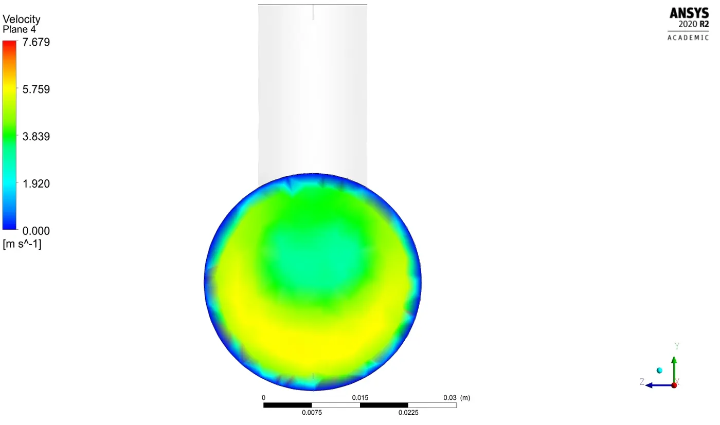 |
 |
|
| 0.25 | Temperature | 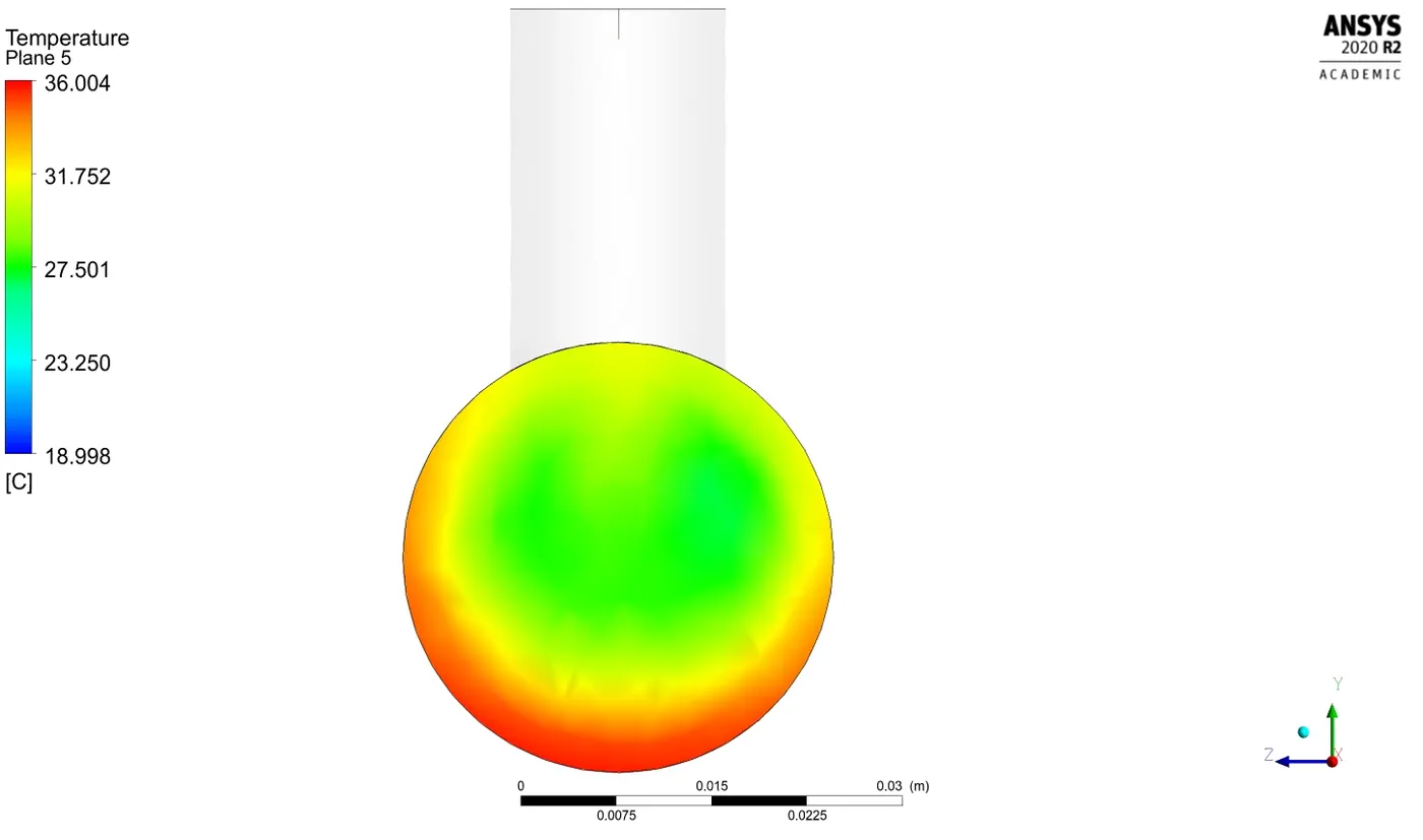 |
 |
| Velocity | 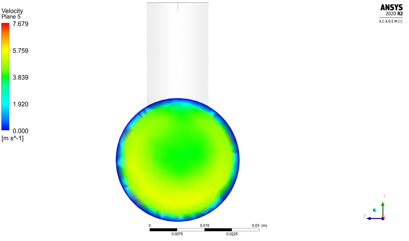 |
 |
|
| 0.3 | Temperature | 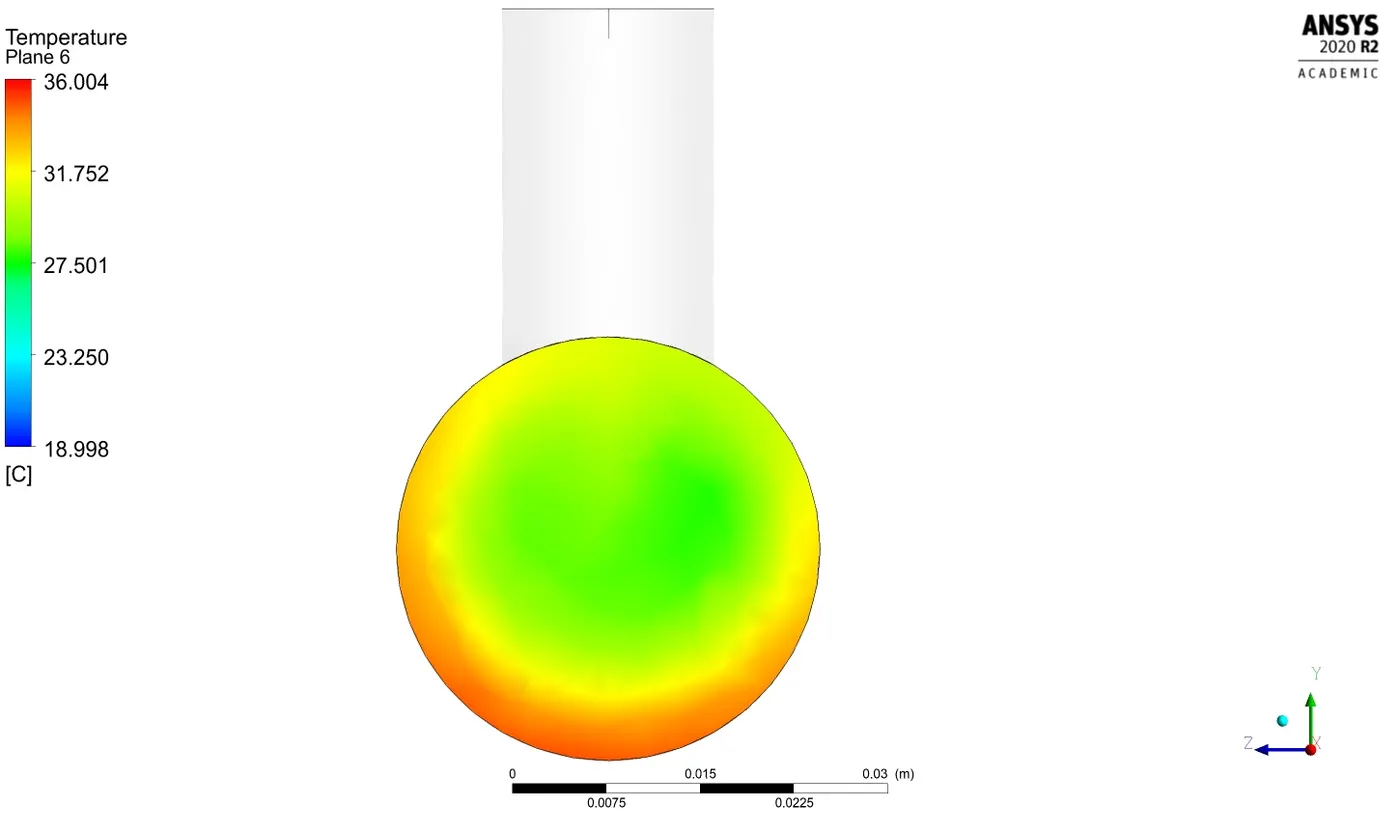 |
 |
| Velocity | 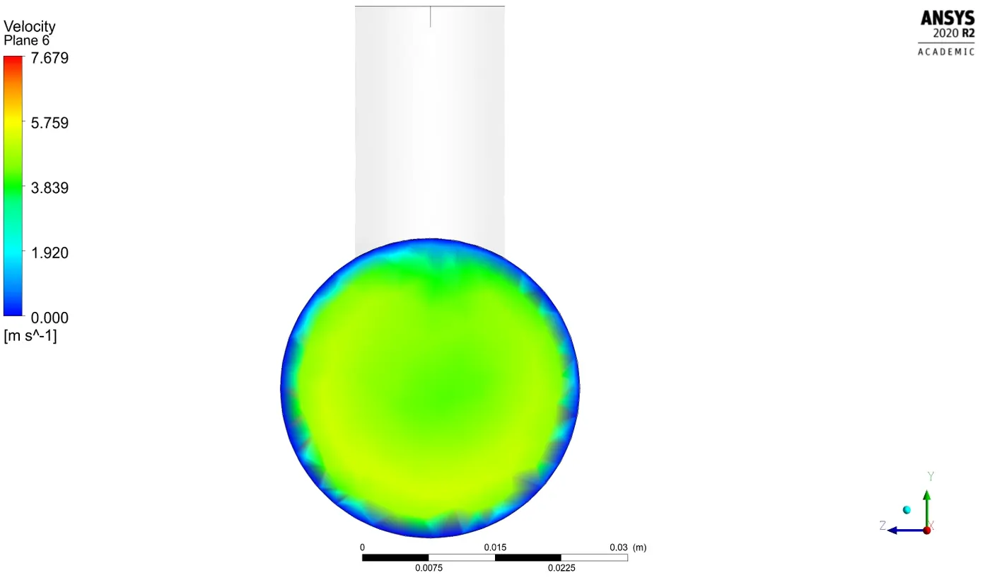 |
 |
|
| 0.35 | Temperature | 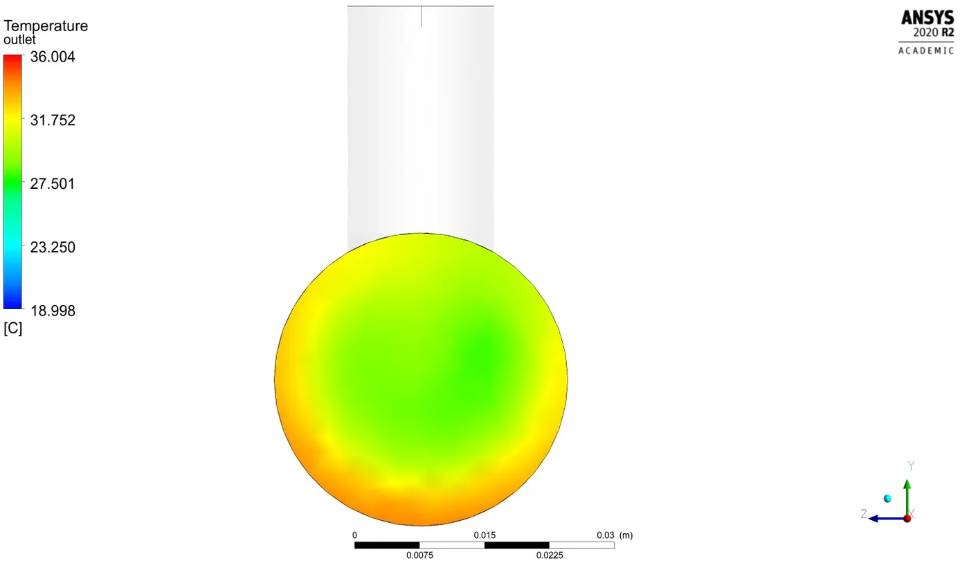 |
 |
| Velocity | 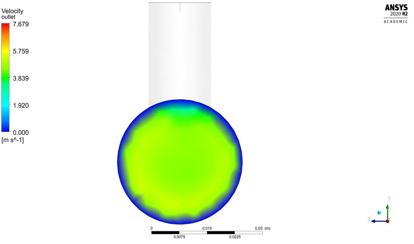 |
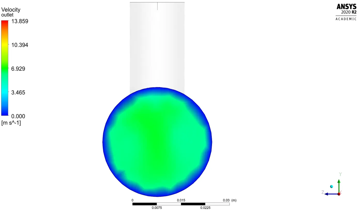 |
Fig.4.2. Long Pipe Cross-Sectional Temperature and Velocity Contours
From the tabulations for case 1 (short pipe), the average outlet temperature obtained was approximately 30.3°C with a standard deviation of 2°C when the inlet momentum ratio was 2. When the momentum ratio was 4 in the same case, the average outlet temperature and the standard deviation was approximately 27.6 °C and 1.2 °C respectively.
When the momentum ratio is doubled, the average outlet temperature’s difference was approximately 3°C. This shows that average outlet temperature decreases with increased momentum ratio. When the length of the pipe was increased, the average temperature reduced by approximately 0.2°C. This shows that long pipe allows more mixing of fluids with different temperatures for uniform average outlet temperature.
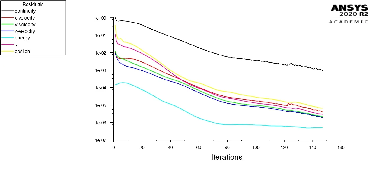
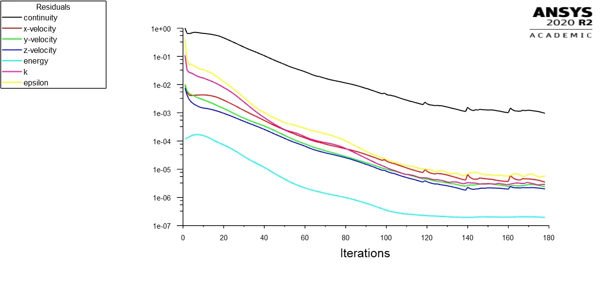
The convergence plot for the short pipe using K - Epsilon Realizable model equations against the momentum ratios and mesh size are shown. In low momentum ratio, the residuals dropped at high rate and attained convergence value till the calculation was completed. But in high momentum ratio, the residuals gradually reduced and attained convergence till the calculation was completed. The change in mesh size had no effect in the rate of reduction of residuals.
| Mesh Size (m) | Low Momentum Ratio | High Momentum Ratio |
| 0.004 | 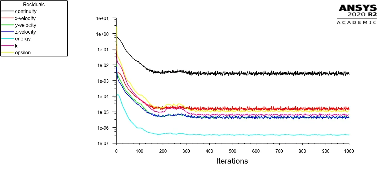 |
 |
| 0.003 | 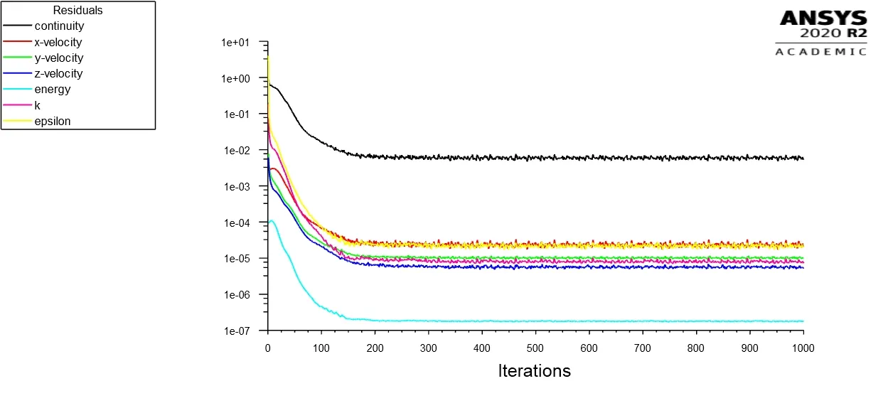 |
 |
| 0.002 | 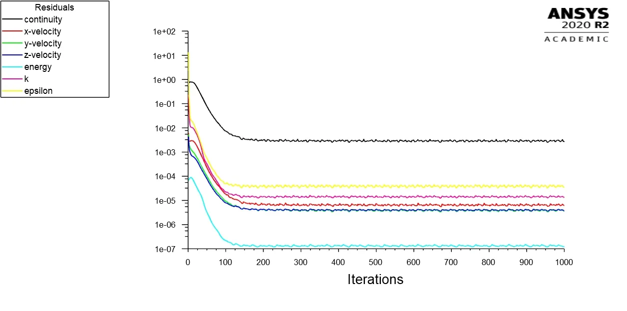 |
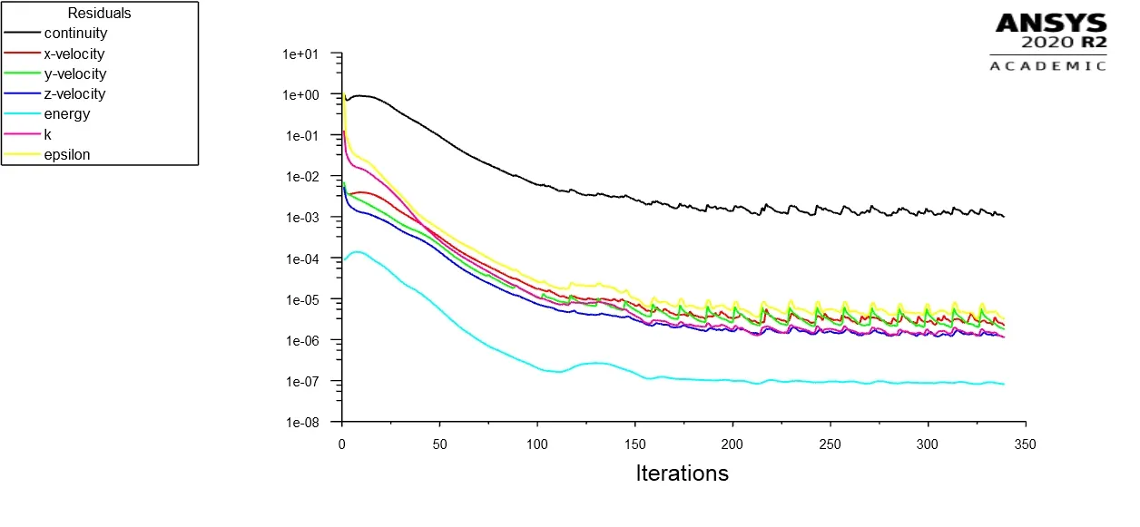 |
Fig.4.3. Short Pipe Convergence Plot (K-ε Realizable)
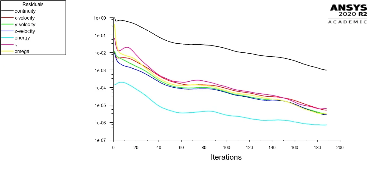
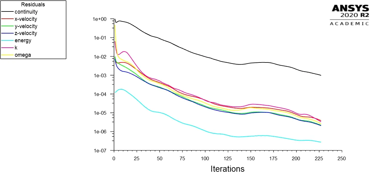
The convergence plot for the short pipe using K - Omega SST model equations against the momentum ratios and mesh size are shown. In low momentum ratio, the residuals dropped gradually and attained convergence value till the calculation was completed. The same plot was observed in high momentum ratio except in finer mesh size of 0.002 m. In the finer mesh at high momentum ratio, the residuals dropped quickly reduced and fluctuated till the calculation was completed. The change in mesh size had small effect in the rate of reduction of residuals.
| Mesh Size (m) | Low Momentum Ratio | High Momentum Ratio |
| 0.004 | 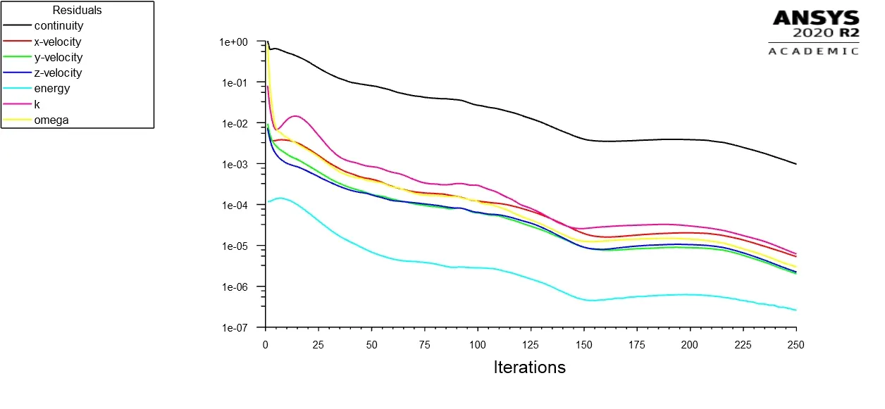 |
 |
| 0.003 | 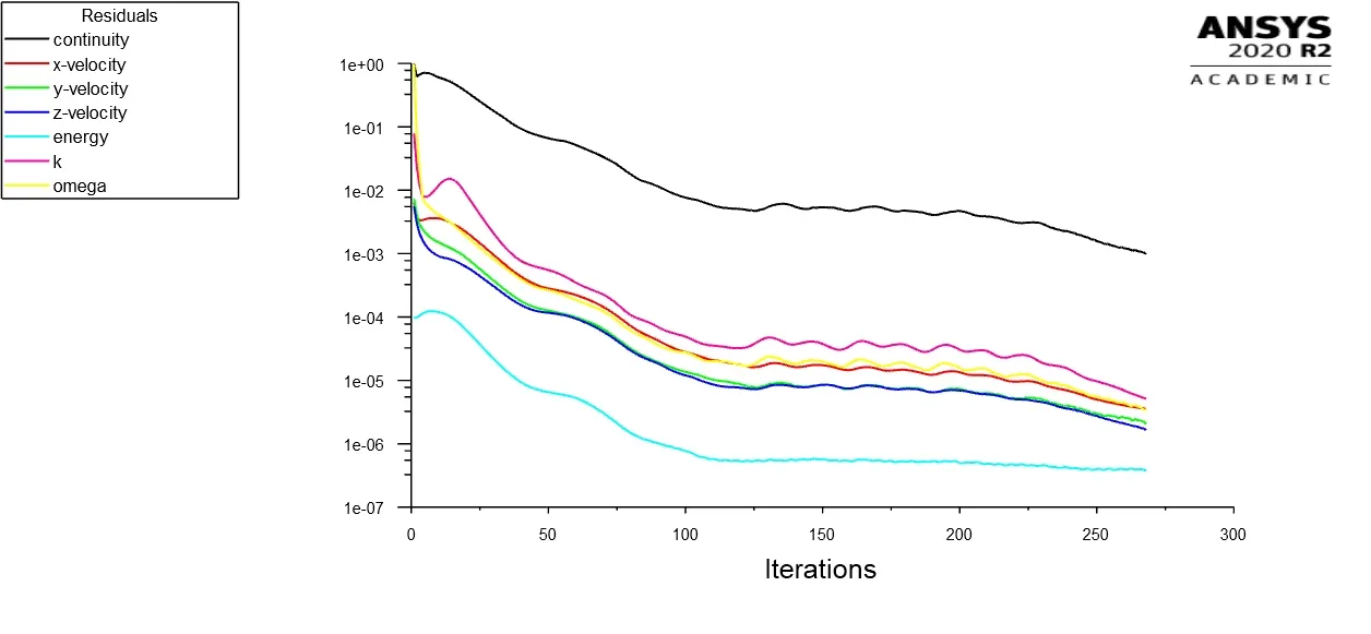 |
 |
| 0.002 | 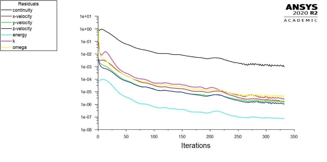 |
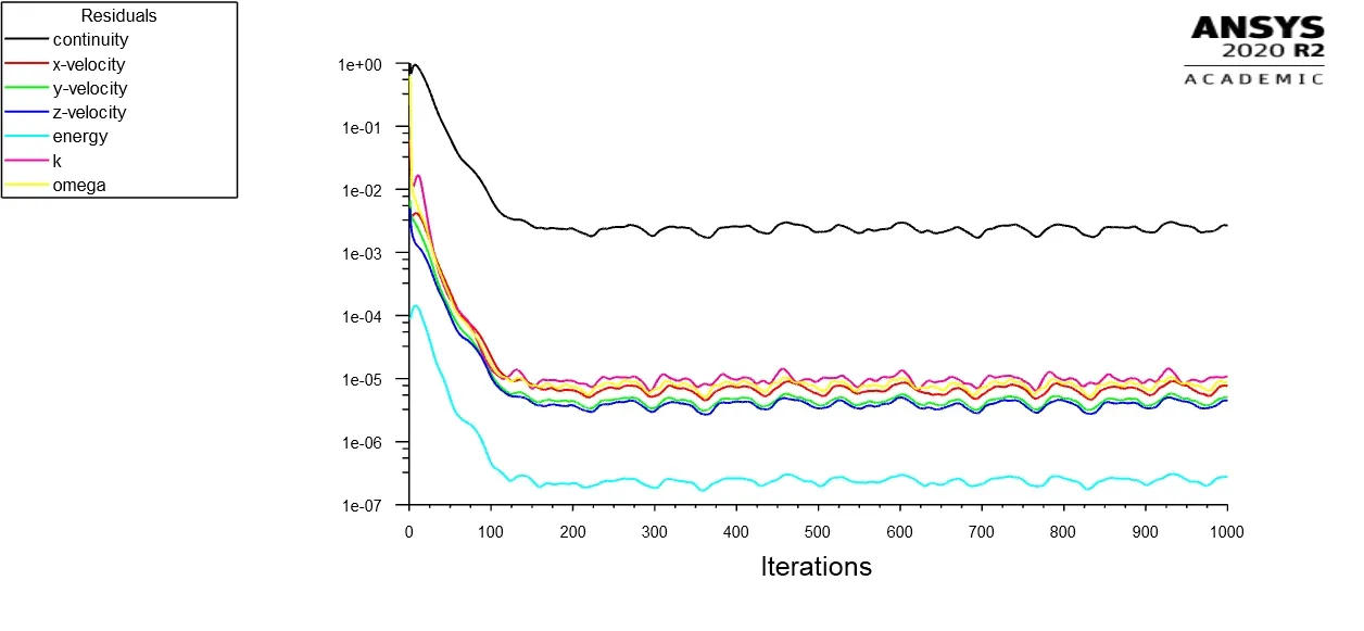 |
Fig.4.4. Short Pipe Convergence Plot (K-Ω SST)
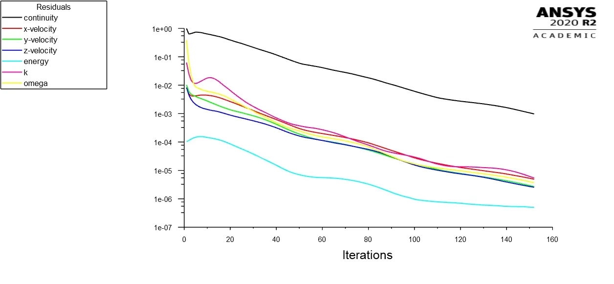
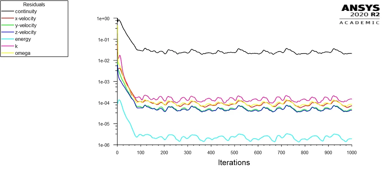
The convergence plot for the long pipe using K - Omega SST model equations against the momentum ratios and mesh size are shown. In low momentum ratio, the residuals dropped gradually and attained convergence value till the calculation was completed. The same plot was observed in high momentum ratio except in finer mesh sizes of 0.003 m and 0.002 m. In both of the finer mesh at high momentum ratio, the residuals dropped quickly reduced and fluctuated till the calculation was completed. The fluctuation was at lower frequency in mesh size of 0.002 m than mesh size of 0.003 m. The change in mesh size had visible effect in the rate of reduction of residuals.
| Mesh Size (m) | Low Momentum Ratio | High Momentum Ratio |
| 0.004 | 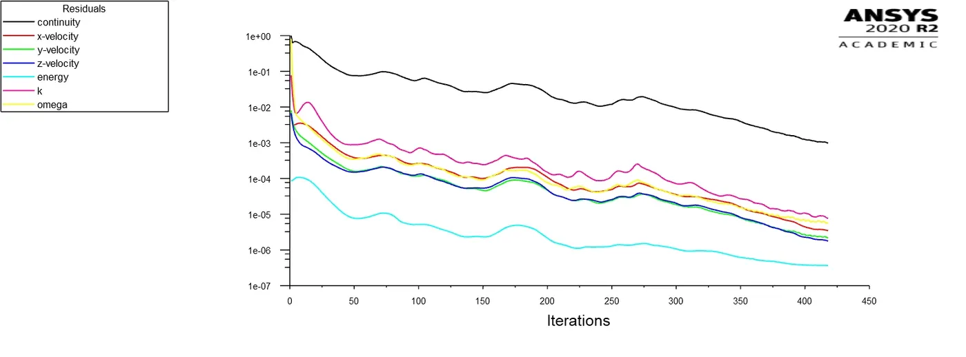 |
 |
| 0.003 | 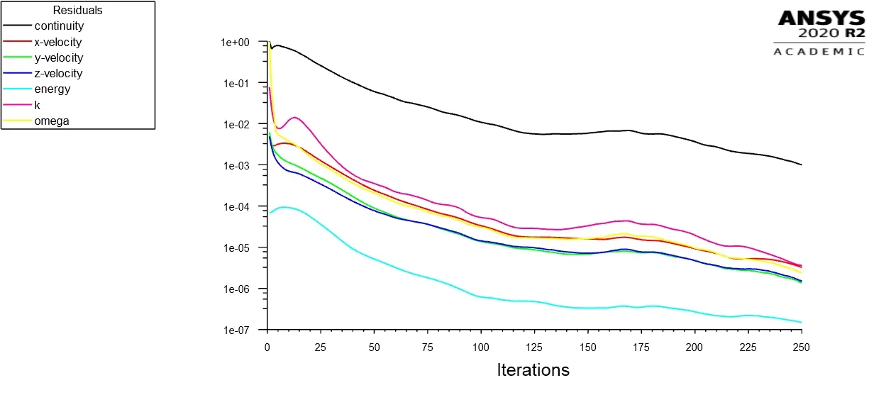 |
 |
| 0.002 | 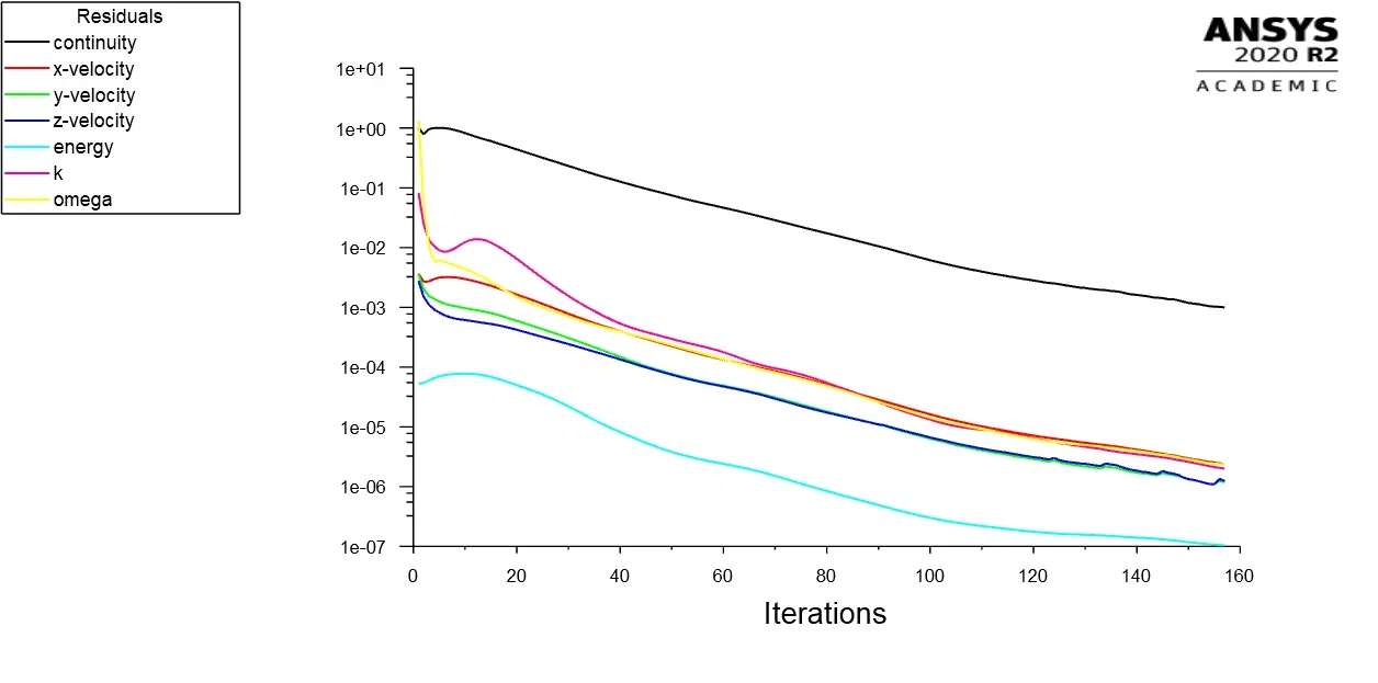 |
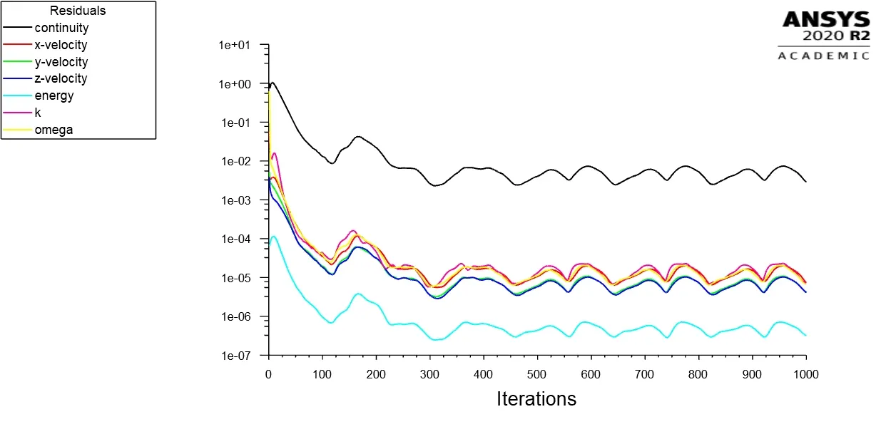 |
Fig.4.5. Long Pipe Convergence Plot (K-Ω SST)
8. Conclusion
In both cases, three different mesh sized were used to obtain sharp temperature contours in the model given. The K-Omega SST model equation was chosen for case 2 as it provided the temperature contours at the boundary wall, which provided more insight in the mixing tee.
The long pipe provided more mixing of fluids, which led to uniform averaged temperature at the outlet without the influence of the hot fluid. The standard deviation of temperature graph fluctuated in case 2, when the mesh quality was improved (from coarse to fine).
If the mixing tee is used for HVAC or other systems, its recommended to use long pipe as it provides good mixing of fluids at different temperatures.