Independent Research Project

COMPUTATIONAL INVESTIGATION OF INTAKE SYSTEM OF TURBOFAN’S INSTAKE SYSTEM

1. INTRODUCTION

Jet propulsion engine is a class of power-developing thermodynamic machines based on the Brayton cycle. Jet propulsion came into existence since the Wright Brothers invented the first aircraft, which started with the use of an Internal Combustion (IC) engine and has advanced to a stage where multiple compressors are being deployed to burn the aviation fuel using atmospheric air.
At present, ideal jet propulsion manipulates the high velocity of the aircraft to suck the atmospheric air with the use of intake fans. The intake fans, compressors, and turbines are designed by utilizing certain airfoil profiles having high camber angle, to obtain high fluid flow. The jet engine is designed to run by single or multiple shafts, resulting in varying speeds to the intake fan, compressors, and turbine, resulting in higher efficiency.

2. OBJECTIVE

To simulate the intake system - rotating fan’s blade models within its real-time working scenarios to determine pressure and velocity drops and their effects on bypass ratio and efficiency.

3. 3D MODEL

The rotational fan blade models of 1:2 scale are made up of two aero-foils (A18 smoothed and AH 7876) having a blade diameter of 1.53 m. A single fluid volume is created for the stationary model and two fluid volumes (rotational and stationary) were created for the rotational model for the simulations.

Table 3.1: Rotating Fan Design Parameters

METRICS	VALUE
FAN DIAMETER	1.53 m
NO OF BLADE	21
TIP VELOCITY	724.205 mph
BYPASS RATIO	9.53
MACH	0.89
ALTITUDE	40,000 ft

Table 3.2: Aerofoil Design Parameters - Model 1

PARAMETERS	A - 18 SMOOTHED	AH 7476
CHORD LENGTH	0.25 m	0.25 m
SCALE X	0 m	0.125 m
SCALE Y	0 m	0.125 m
ANGLE OF INCIDENCE	20 deg	15 deg

Table 3.3: Aerofoil Design Parameters - Model 2

PARAMETERS	A - 18 SMOOTHED	AH 7476
CHORD LENGTH	0.25 m	0.25 m
SCALE X	0 m	0.125 m
SCALE Y	0 deg	15 deg
ANGLE OF INCIDENCE	10 deg	15 deg

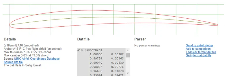
Fig.3.1. Aerofoil A-18 (Smoothed)

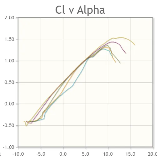
Fig.3.2. Aerofoil A-18 Smoothed C_L v α Graph

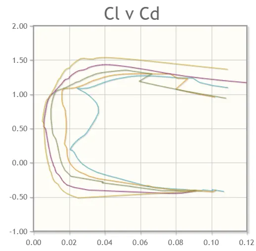
Fig.3.3. Aerofoil A-18 Smoothed C_L v C_D Graph

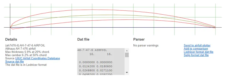
Fig.3.4. Aerofoil AH7476

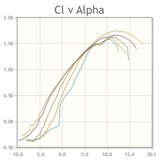
Fig.3.5. Aerofoil AH7476 Smoothed C_L v α Graph

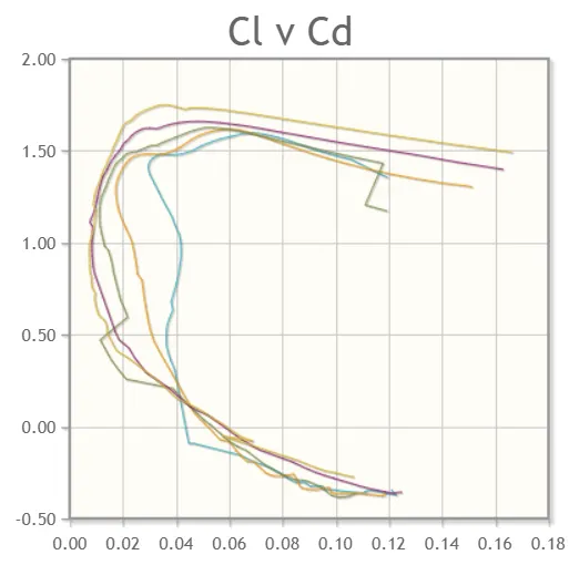
Fig.3.6. Aerofoil AH7476 Smoothed C_L v C_D Graph

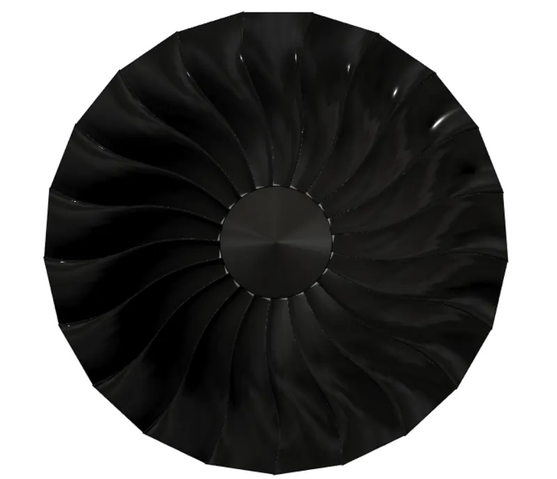
Fig.3.7. Rotating Fan Model 1

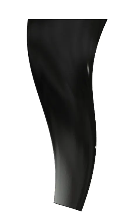
Fig.3.8. Rotating Fan Single Blade Model 1

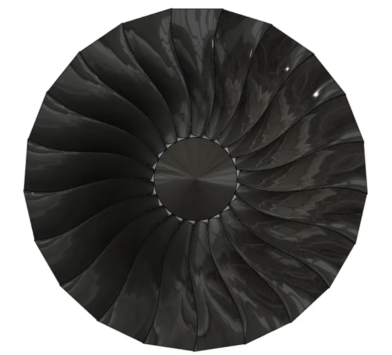
Fig.3.9. Rotating Fan Model 2

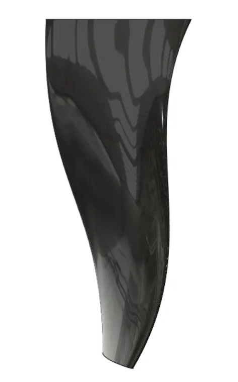
Fig.3.10. Rotating Fan Single Blade Model 2

Table 3.4: Fluid Volume Data

PARAMETERS	ROTATING VOLUME	STATIONARY VOLUME
ANGLE 1	15.5 deg	15.5 deg
ANGLE 2	18.786 deg	18.786 deg
RADIUS	0.8 m	2 m
DISTANCE FROM BLADE	-0.01 m to 0.25 m	-1 m to 4 m

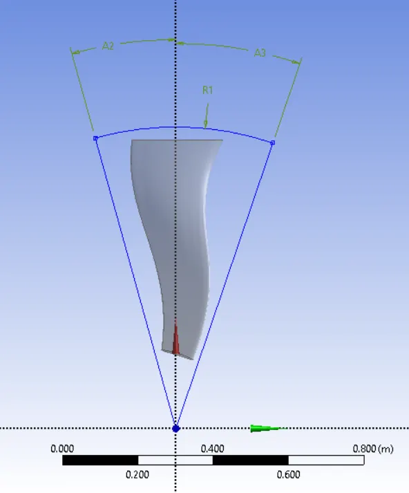
Fig.3.11. Rotating Volume - Sketch View

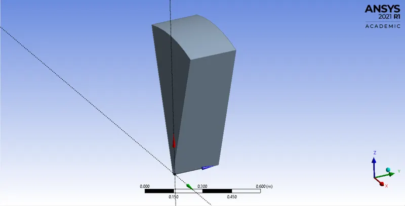
Fig.3.12. Rotating Volume - Isometric View

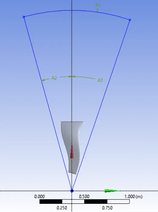
Fig.3.13. Stationary Volume - Sketch View

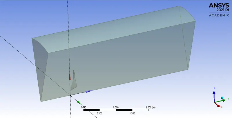
Fig.3.14. Stationary Volume - Isometric View

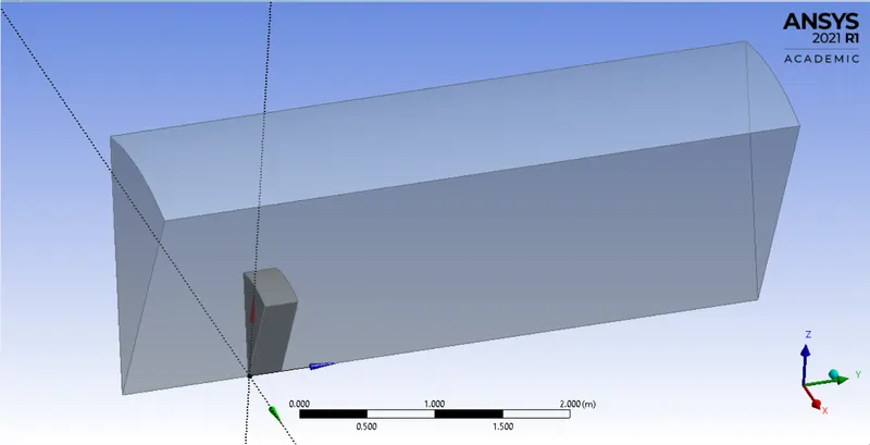
Fig.3.15. Fluid Volume - Shaded Volume View

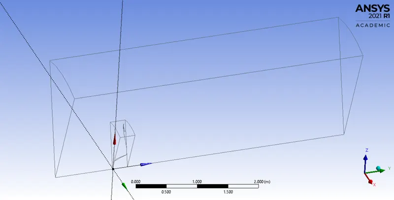
Fig.3.16. Fluid Volume - Wire Frame View

4. MESH DETAILS

Simple mesh metrics are used to obtain a good mesh that could run in the Ansys Student version. A fine mesh having various mesh metrics would result in excessive elements being run using Ansys full version in a higher computational power.

4.1. MESH

Table 4.1.1: Mesh Details

METRICS	VALUE
ALGORITHM	PATCH CONFIRMING
MESH METHOD	TETRAHEDRONS
BODY SIZING (ROTATING VOLUME)	2.75e-2 m
BODY SIZING (STATIONARY VOLUME)	5e-2 m
NODES (MODEL 1)	79697
ELEMENTS (MODEL 1)	433384
NODES (MODEL 2)	79610
ELEMENTS (MODEL 2)	433082

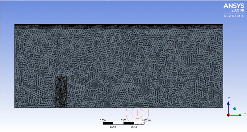
Fig.4.1.1. Mesh - Side View

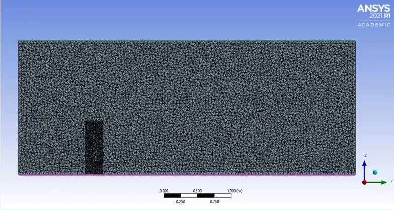
Fig.4.1.2. Mesh- Sectional View

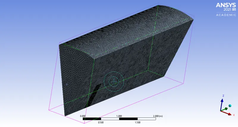
Fig.4.1.3. Mesh - Isometric View

4.2. MESH CHART

4.2.1. ELEMENT QUALITY

Element quality is said to be good if the effects due to application, boundary value problem, and element type are beneficial. In model 1, the average mesh element quality of 0.85 is attained, having a minimum and maximum mesh element quality of 0.16 and 1.0 respectively. In model 2, the average mesh element quality of 0.85 is attained, having a minimum and maximum mesh element quality of 0.03 and 1.0 respectively.

Table 4.2.1.1: Element Quality - Model 1

METRICS	VALUE
MIN	0.15878
MAX	1.0
AVERAGE	0.84897
STANDARD DEVIATION	9.4161e-002

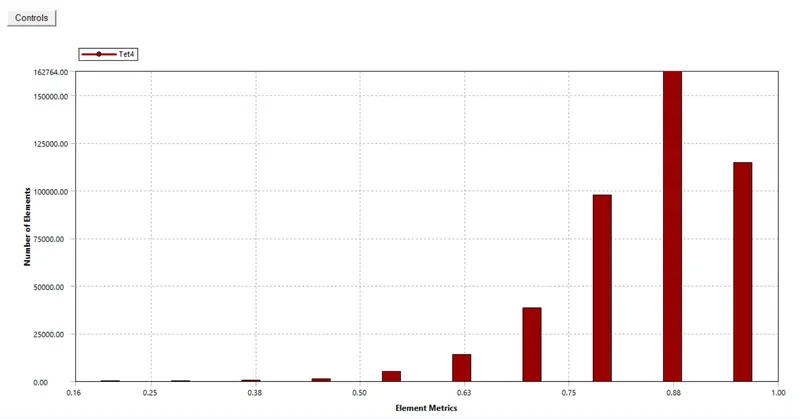
Fig.4.2.1.1. Element Quality - Model 1

Table 4.2.1.2: Element Quality - Model 2

METRICS	VALUE
MIN	3.2141e-002
MAX	1.0
AVERAGE	0.84941
STANDARD DEVIATION	9.4712e-002

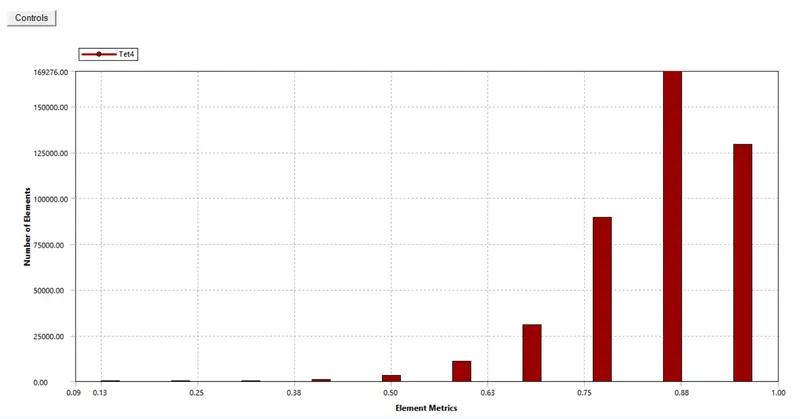
Fig.4.2.1.2. Element Quality - Model 2

4.2.2. ORTHOGONAL QUALITY

Mesh orthogonality relates how close the angle between adjacent element faces or edges is to some optimal angle. A high number of elements had good to outstanding orthogonal quality, which provided another quality check to proceed with for CFD.

In model 1, the average mesh orthogonal quality of 0.79 is obtained, having a minimum and maximum mesh orthogonal quality of 0.11 and 0.99 respectively. In model 2, the average mesh orthogonal quality of 0.79 is attained, having a minimum and maximum mesh orthogonal quality of 0.015 and 0.99 respectively.

Table 4.2.2.1: Orthogonal Quality - Model 1

METRICS	VALUE
MIN	0.11129
MAX	0.99669
AVERAGE	0.78925
STANDARD DEVIATION	0.1149

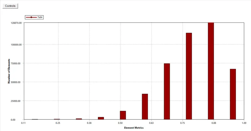
Fig.4.2.2.1. Orthogonal Quality - Model 1

Table 4.2.2.2: Orthogonal Quality - Model 2

METRICS	VALUE
MIN	1.5198e-002
MAX	0.99577
AVERAGE	0.79001
STANDARD DEVIATION	0.11548

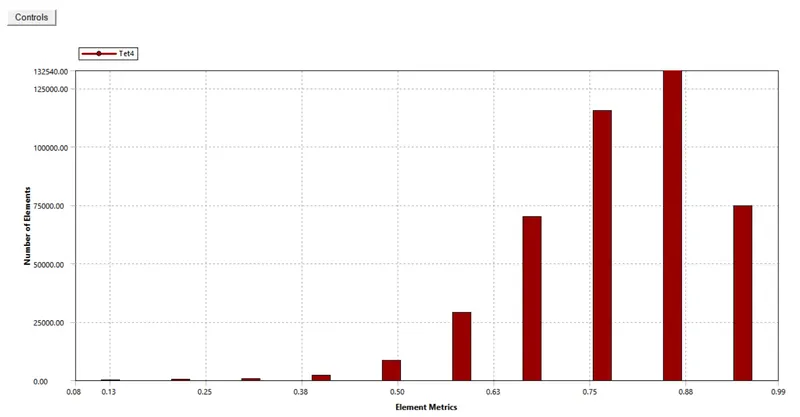
Fig.4.2.2.2. Orthogonal Quality - Model 2

4.2.3. SKEWNESS

A high number of elements had high skewness quality, which determines the percentage of smoothness of the elements. This quality check provided the final reason to proceed with the mesh obtained for CFD.

In model 1, the average mesh skewness quality of 0.21 is obtained, having a minimum and maximum mesh skewness quality of 7.99e-8 and 0.89 respectively. In model 2, the average mesh skewness quality of 0.21 is attained, having a minimum and maximum mesh skewness quality of 6.64e-7 and 0.98 respectively.

Table 4.2.3.1: Skewness Quality - Model 1

METRICS	VALUE
MIN	7.9936e-008
MAX	0.88871
AVERAGE	0.2095
STANDARD DEVIATION	0.11646

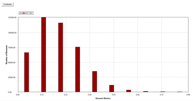
Fig.4.2.3.1. Skewness - Model 1

Table 4.2.3.2: Skewness Quality - Model 2

METRICS	VALUE
MIN	6.4652e-007
MAX	0.9848
AVERAGE	0.20871
STANDARD DEVIATION	0.11707

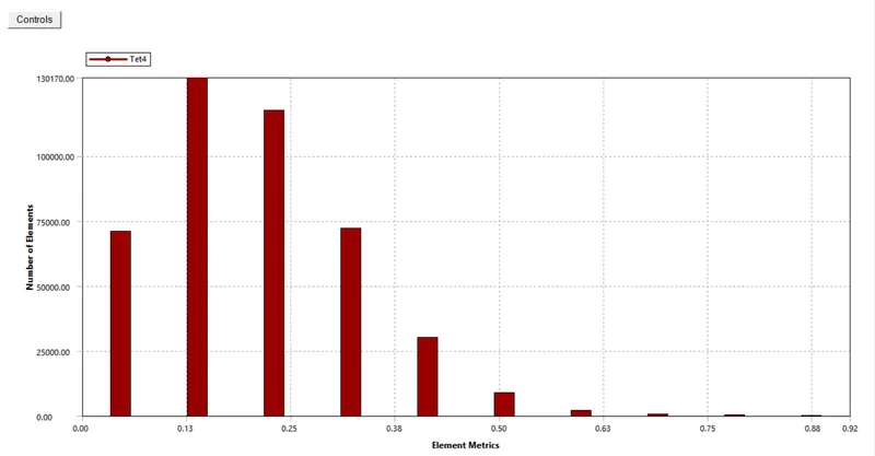
Fig.4.2.3.2. Skewness - Model 2

5. THEORETICAL CALCULATIONS

5.1. PARAMETERS

Altitude (z) = 40,000 ft = 12,192 m

Mach (M) = 0.89

Blade Radius (r) = 0.765 m

Blade tip velocity (v) = 724.205 mph = 323.749 m/s

5.2. FORMULAE

M = c/a

v = ωr

5.3. CALCULATION

For z = 12,192 m,

P = 0.187624 bar

ρ = 0.30236 kg/m³

a = 295.2 m/s

μ = 14.17×10^-6 N-s/m²

T = 216.65 K

c = M×a = (0.89)(295.2) = 262.728 m/s

ω = v/r = 323.749/0.765 = 423.201 rad/s

6. MATERIAL PROPERTIES

Material properties of fluid were obtained according to the cruising specifications of the turbofan using standard air properties against altitude.

Table 6.1: Material Properties

MERICS	VALUE
MATERIAL	AIR
DENSITY	0.30236 kg/m3
VISCOSITY	14.17×10-6 N-s/m2

7. BOUNDARY CONDITIONS

Due to the excessive angular velocity of the blade, the time step was reduced to 0.1 micro-second for 200 iterations such that a single rotation of the blade is achieved.

Table 7.1: Boundary Conditions

METRICS	VALUE
INLET VELOCITY	262.728 m/s
ANGULAR VELOCITY	423.201 rad/s
VISCOUS MODEL	K-EPSILON REALIZABLE
NEAR WALL TREATMENT	SCALABLE WALL FUNCTIONS
SOLVER	TRANSIENT
TIME STEP	0.0001 sec
ITERATIONS	200

8. RESULTS

Five line geometries are created at different equal intervals from the blade region. The pressure and velocity values at various lines were obtained at a height of 0.15 m from the blade’s rotational axis.

Table 8.1: Line Geometry

LINES	DISTANCE (m)
LINE 1	-0.35
LINE 2	0.35
LINE 3	0.70
LINE 4	1.05
LINE 5	1.40

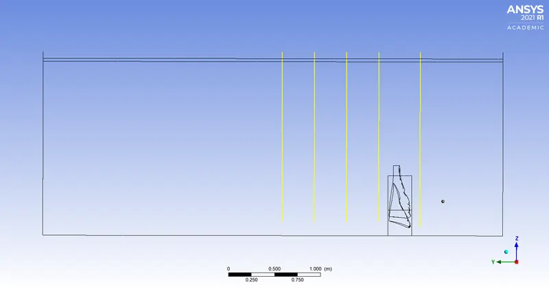
Fig.8.1. Line Geometry

8.1. SCALED RESIDUALS

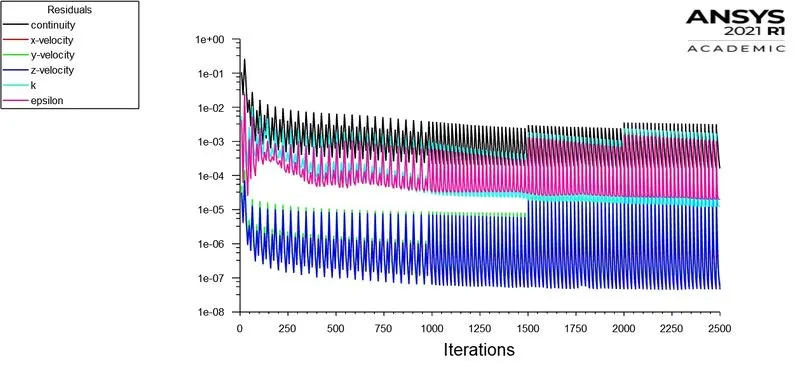
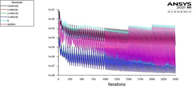
The residuals tended to fluctuate in both models, till the calculation was completed or encountered the floating-point error. Convergence of residuals was not obtained as calculation was done for 125 time-steps.

Fig.8.1.1. Scaled Residuals - Model 1	Fig.8.1.2. Scaled Residuals - Model 2

8.2. MASS FLOW RATE

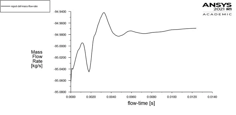
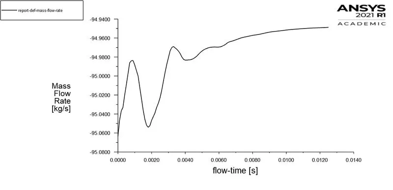
Mass flow rate at 0.35m behind the blade varied until a flow time of 0.009 seconds in models 1 and 2 respectively. The reported mass flow rate in model 1 and 2 were -94.969 kg/s and -94.949 kg/s respectively. In model 1, the mass flow rate peak was observed at 0.003 seconds having approximately equal value to the final report. In model 2, the mass flow rate peak was observed beyond the fluctuations.

Fig.8.2.1. Mass Flow Rate - Model 1	Fig.8.2.2. Mass Flow Rate - Model 2

8.3. COEFFICIENT OF LIFT

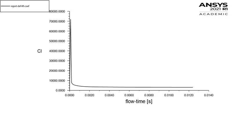
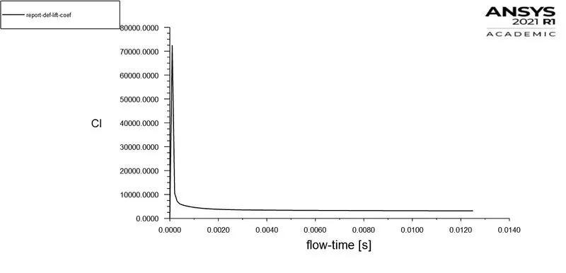
The coefficient of lift depicts the amount of lift generated by the blade due to the fluid flow. In both models, the coefficient of lift drastically drops and converges at 5000 indicating a constant lift coefficient while high-speed rotation.

Fig.8.3.1. Coefficient of Lift - Model 1	Fig.8.3.2. Coefficient of Lift - Model 2

8.4. COEFFICIENT OF DRAG

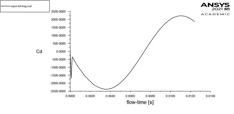
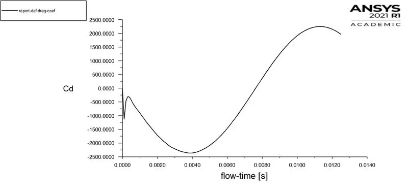
The coefficient of drag depicts the resistance encountered by the blade against the fluid flow. In both models, the coefficient of drag oscillates at an amplitude of 2250 and a period of 0.00735 seconds after drastically increasing to 0.

Fig.8.4.1. Coefficient of Drag - Model 1	Fig.8.4.2. Coefficient of Drag - Model 2

8.5. PRESSURE CONTOURS

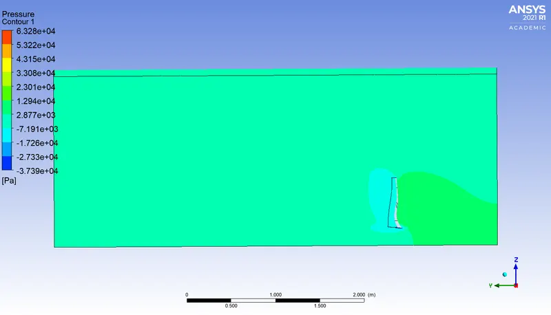
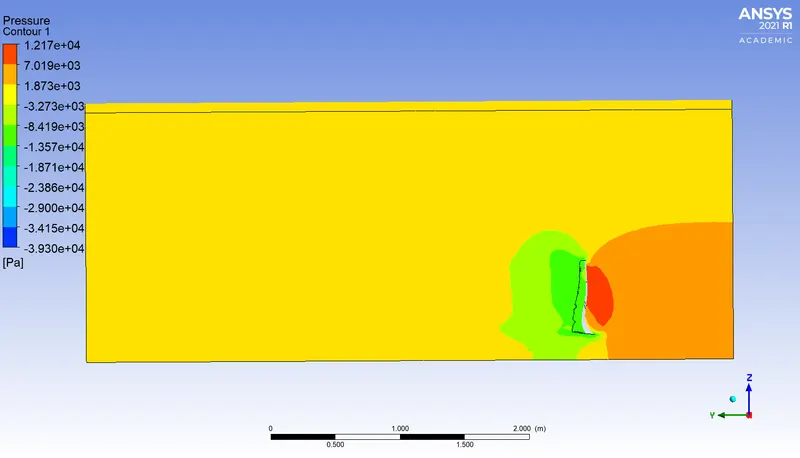
Pressure contours portray the pressure regions in the fluid volume along the Y-Z plane. In both models, a decrease in pressure relative to the inlet is observed as calculated inlet pressure had not been implemented. In model 1, the pressure region ranged from 6.328×10⁴ Pa to -3.739×10⁴ Pa while in model 2, the pressure region ranges from 1.217×10⁴ Pa to -3.930×10⁴ Pa.

The decrease in pressure behind the blade extends over a large region in model 1 than in model 2 due to the effect of the secondary low-velocity region. The high pressure at the leading edge of the blade allows a laminar flow of the fluid during the blade’s rotation. The pressure drop near the blade’s bottom allows a laminar flow to the combustion chamber via the stationary fan.

Fig.8.5.1. Pressure Contours - Model 1	Fig.8.5.2. Pressure Contours - Model 2

8.6. PRESSURE DROP

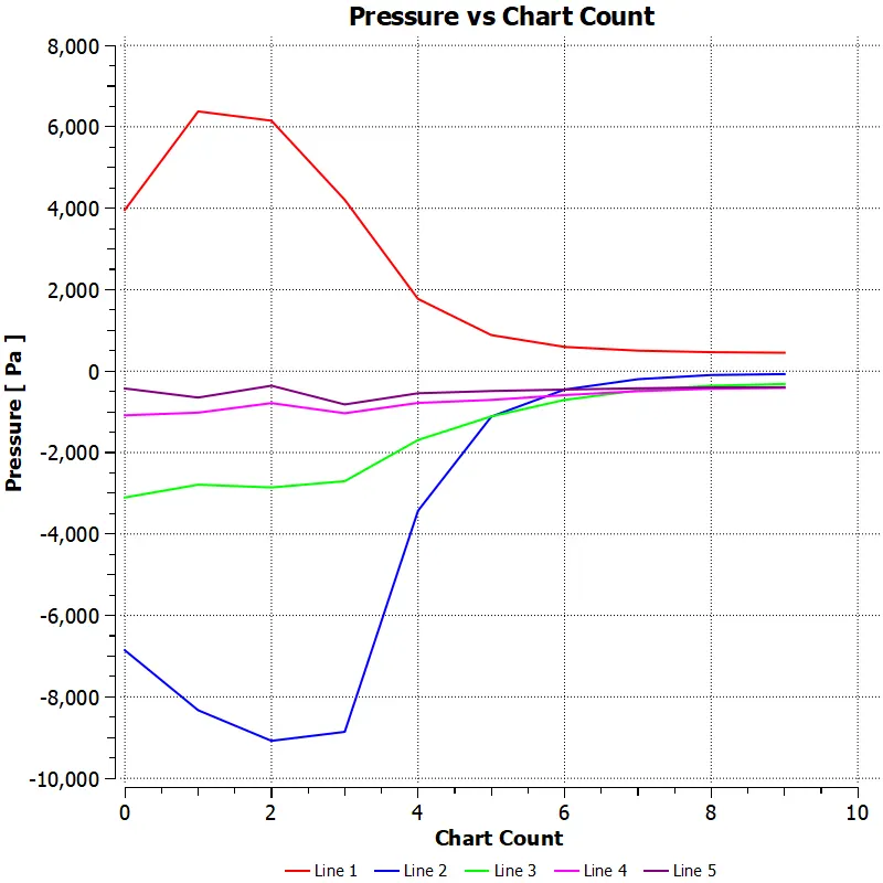
The pressure drop beyond the blade in both models is similar, resulting in a reduced difference in the effect of the blade on pressure. The need for a drop in pressure behind the blade is achieved for cooling purposes.

Table 8.6.1: Pressure Drop

LINE	PRESSURE (Pa)
	MODEL 1	MODEL 2
LINE 1	6564.32	4523.32
LINE 2	-8623.43	-8307.3
LINE 3	-2803.9	-3412.81
LINE 4	-957.848	-1431.5
LINE 5	-594.074	-440.124

Fig.8.6.1. Pressure Drop Chart - Model 1	Fig.8.6.2. Pressure Drop Chart - Model 2

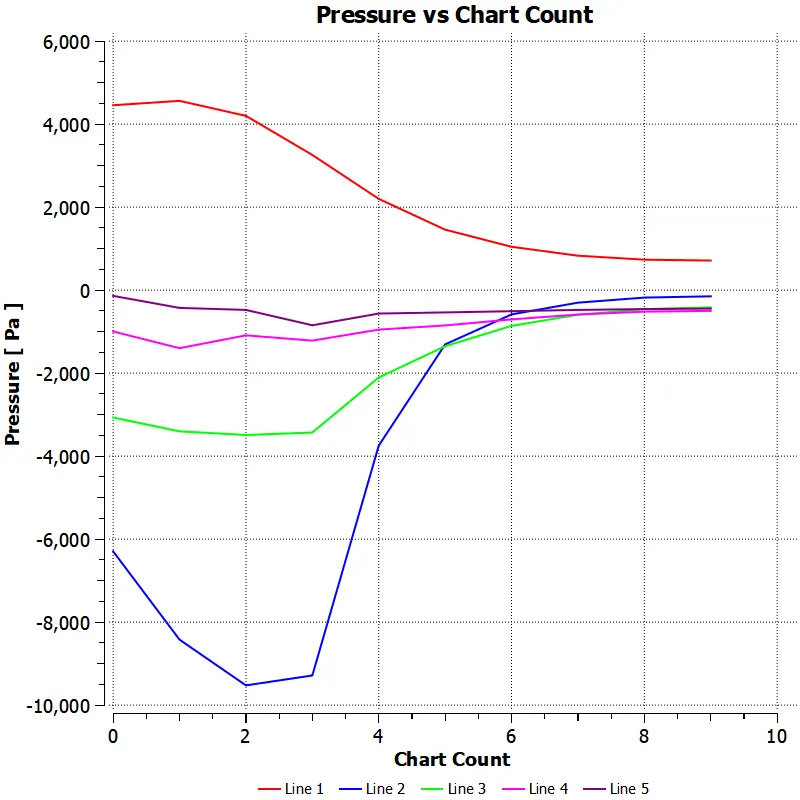
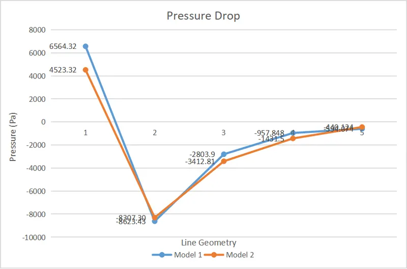
Fig. 8.6.3. Pressure Chart - Comparison

8.7. VELOCITY CONTOURS

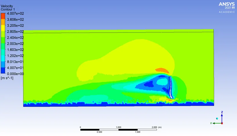
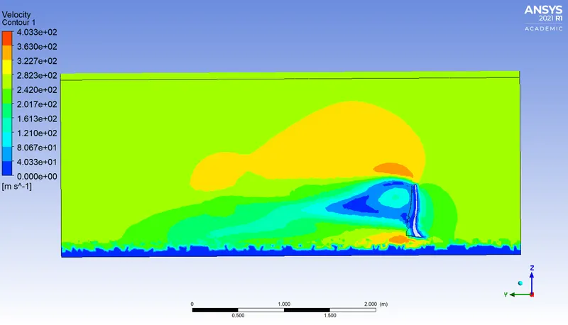
Velocity contours portray the velocity regions on fluid volume in open environmental conditions along the Y-Z plane. In both models, a decrease in velocity indicated the action of the blade’s shape on the fluid flow, which is expected. In model 1, velocity ranges from 400.7 - 40.07 m/s while in model 2, the velocity ranges from 403.3 - 40.33 m/s.

The decrease in velocity above the blade’s bottom is higher in model 1 than in model 2. A secondary low and high-velocity contours are present near the blade’s bottom region in model 1 and model 2 respectively. The increase in velocity near the blade’s bottom in model 2 than in model 1 allows a higher mass flow rate to the combustion chamber through the stationary fan.

Fig.8.7.1. Velocity Contours - Model 1	Fig.8.7.2. Velocity Contours - Model 2

8.8. VELOCITY DROP

The velocity drop beyond the blade is greater in model 1 than in model 2. The need for a lower velocity beyond the blade’s top region allows a stagnant velocity for the cooling process while higher velocity beyond the blade’s bottom region allows a higher mass flow rate for combustion via intermediate pressure turbines.

Table 8.8.1: Velocity Drop

LINE	VELOCITY (m/s)
	MODEL 1	MODEL 2
LINE 1	245.28	245.193
LINE 2	75.213	112.832
LINE 3	113.477	163.704
LINE 4	166.431	199.995
LINE 5	195.884	180.528

Fig.8.8.1. Velocity Drop Chart - Model 1	Fig.8.8.2. Velocity Drop Chart - Model 2

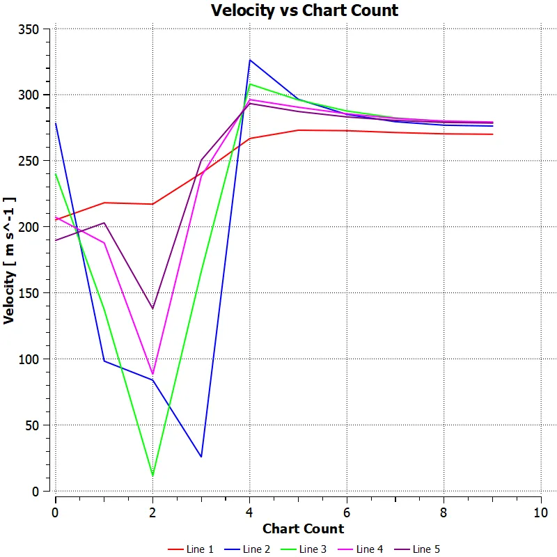
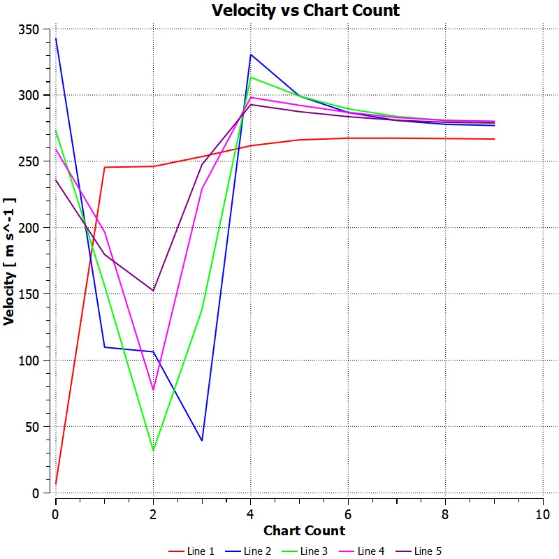
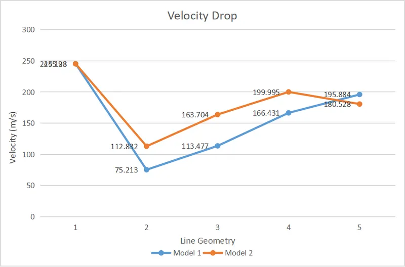
Fig. 8.8.3. Velocity Chart - Comparison

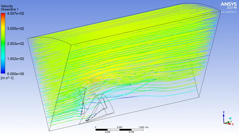
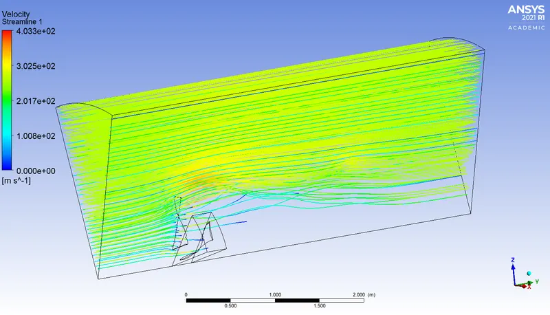
8.9. VELOCITY STREAMLINES

Velocity streamlines portray the direction and magnitude of fluid flow’s velocity. For model 1, the vectors attain 400.7 - 100.2 m/s while for model 2, the vectors attain 403.3 - 100.3 m/s. This is due to the existence of various pressure regions around the blade.

In model 1, the fluid curves along the blade’s profile having no reverse flow. In model 2, the fluid curves along with the blade’s profile while having negligible reverse flow. The streamlines’ convergence is higher in model 1 than in model 2, resulting in a higher mass flow rate behind the blade’s top region.

Fig.8.9.1. Velocity Streamlines - Model 1	Fig.8.9.2. Velocity Streamlines - Model 2

9. CONCLUSION

Laminar flow under turbofan’s working conditions for both rotating fan’s single blade models was attained, resulting in higher undesired velocities due to the open environment.

Temperature and pressure as an inlet condition were not used as it leads to floating-point error and abrupt stoppage of the simulation.

An increase of velocity beyond the blade’s bottom region results in an increase in mass flow rate for combustion leading to a decrease in bypass ratio.

Decrease in the angle of attack for the bottom aerofoil results in the increase of velocity behind the blade’s bottom region. This could improve the efficiency of the turbofan.

10. REFERENCES

A18 (smoothed) (a18sm-il) (airfoiltools.com)

AH-7-47-6 AIRFOIL (ah7476-il) (airfoiltools.com)