Week 5 - Rayleigh Taylor Instability
RAYLEIGH TAYLOR INSTABILITY SIMULATION
1. OBJECTIVE
To perform Rayleigh Taylor instability simulation for two different mesh sizes, and to run a simulation with water and user-defined material.
2. 2D MODEL
A 2-D model, consisting of two zones, is used for the Rayleigh Taylor instability simulation. The zones are obtained by using pull feature, to provide a surface model.
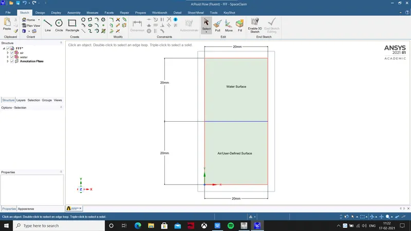
Fig.2.1. 2-D Surface Model
3. COMPUTATIONAL MODEL
Rayleigh-Taylor Instability
The Rayleigh–Taylor (RT) instability deals with the interface instability between two viscous fluids having different densities and dynamic viscosity. The practical CFD models which are based on RT waves are:
- Kelvin-Helmholtz instability
This model predicts the onset of instability and transition-to-turbulent flow in fluids having different densities, and moving at various speeds.
- Turbulent Mixing Model
The turbulence Mixing Model is based on multi-phase flow equations, which describe the velocity separation due to the action of a pressure gradient on fluid fragments of different densities. The dissipation due to the drag between the fluid fragments is used as a source of turbulence kinetic energy, which is then used to define turbulent diffusion coefficients.
- Plateau-Rayleigh instability
The Plateau-Rayleigh (PR) instability explains why and how a falling stream of fluid breaks into smaller packets with the same volume, but with less area.
Atwood Number
The Atwood number (A) used in fluid dynamics, is a dimensionless number. It is used in the study of hydrodynamic instabilities in density stratified flows. It’s dimensionless ratio is defined as,
A = (p1-p2)/(p1+p2)
Where, A = Atwood Number
p1 = Density of Heavier Fluid (kg/m3)
p2 = Density of Lighter Fluid (kg/m3)
4. MESH DETAILS
Two different mesh sizes are used to determine the effect of mesh size on the instability simulation.
Table 4.1: Mesh Details 1
|
METRICS |
VALUE |
|
ELEMENT SIZE |
5e-04 |
|
ELEMENTS |
3200 |
|
NODES |
3321 |
Table 4.2: Mesh Details 2
|
METRICS |
VALUE |
|
ELEMENT SIZE |
2e-04 |
|
ELEMENTS |
20000 |
|
NODES |
20301 |
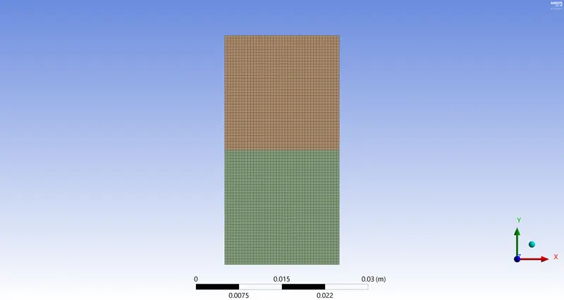
Fig.4.1. Coarse Mesh
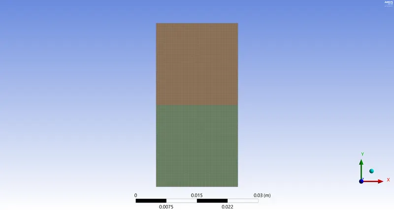
Fig.4.2. Fine Mesh
5. MATERIAL PROPERTIES
Three materials are used for the instability simulations, in which the material with higher density is patched on the upper zone.
Table 5.1: Material 1 Properties
|
METRICS |
VALUE |
|
MATERIAL |
AIR |
|
DENSITY |
1.225 kg/m3 |
|
VISCOSITY |
1.7894e-05 kg/m-s |
Table 5.2: Material 2 Properties
|
METRICS |
VALUE |
|
MATERIAL |
WATER-LIQUID |
|
DENSITY |
998.2 kg/m3 |
|
VISCOSITY |
0.001003 kg/m-s |
Table 5.3: Material 3 Properties
|
METRICS |
VALUE |
|
MATERIAL |
USER-DEFINED |
|
DENSITY |
400 kg/m3 |
|
VISCOSITY |
0.001 kg/m-s |
6. BOUNDARY CONDITIONS
Shared topology is used to bind the zones together, while the edges are considered to be walls.
7. RESULTS
The simulation was done in transient state solution having a time step of 0.005 seconds. The calculation/simulation was done for 500 iterations.
7.1. AIR AND WATER
Steady-state solution cannot be used for RT instability simulation as it doesn’t solve intermediate solution plots w.r.t. time, and it displays the final steady or equilibrium condition.
A = (998.2 - 1.225)/(998.2 + 1.225) = 0.9975
7.1.1. TRANSIENT SOLVER
Animation 7.1.1.1: Air-Water Instability Simulation Transient 1
Animation 7.1.1.2: Air-Water Instability Simulation Transient 2
7.1.2. STEADY SOLVER
Animation 7.1.2.1: Air-Water Instability Simulation Steady
7.2. WATER AND USER-DEFINED MATERIAL
A = (998.2 - 400)/(998.2 + 400) = 0.4278
Animation 7.2.1: Water-User Defined Material Instability Simulation
8. CONCLUSION
The instability of air-water simulation is higher than the water-user defined simulation as the time taken for boundary to develop is very low.
The accuracy of the fluid boundary increases with increase in mesh metrics, providing detailed fluid boundary.
From the two simulations, we observe that the instability of the simulation increases w.r.t the increase of the Atwood number.