Exhaust Port Challenge

EXHAUST PORT – CHT ANALYSIS

1. OBJECTIVE

To simulate the CHT analysis of the given exhaust port using turbulence model, and to calculate the wall/surface heat transfer coefficient on the internal solid surface.

2. 3-D MODEL

The exhaust port consists of four inlets and one outlet perpendicular to the latter. Additional walls are provided near the inlets and outlet for obtaining adiabatic nature.

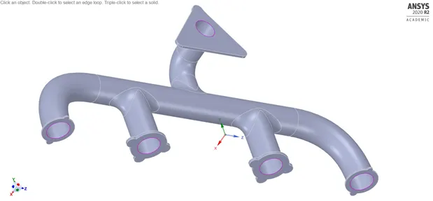
Fig.2.1. Exhaust Port Model

3.COMPUTATIONAL MODEL

The Conjugate Heat Transfer analysis (CHT) is used for the simulation of heat transfer between two or more solid-fluid domains, in which the thermal energy is exchanged. This analysis simultaneously solves all the heat transfer processes in the solid-fluid domain within the model other than using simplified empirical calculations. The CHT analysis is used when heat transfer in the solid-fluid domain is either non-uniform or difficult to calculate empirically.

The verification of HTC predictions from the simulation are done by comparing with a real-time heat transfer experiment of a scaled or exact prototype under the same boundary conditions. The accuracy of HTC values depends upon the quality of mesh obtained, iterations calculated, viscous models and type of solver considered.

The calculations were done for 150 iterations, by having a shared topology between the solid and fluid domains. K-Epsilon Realizable and K-Omega SST viscous models were used to obtain accurate contours of heat transfer coefficient near the solid-fluid boundary.

4. MESH

Table 3.1: Mesh Details

PARAMETERS	SPECIFICATIONS
MESH TYPE	QUAD/TRI
MESH SIZE	0.0075 m
MAXIMUM MESH SIZE	0.015 m
INFLATION LAYERS	5
GROWTH RATE	1.2
MAXIMUM THICKNESS	0.01 m
BODY SIZING	0.015 m
CURVATURE	ON
ELEMENTS	3,29,408
NODES	91,917

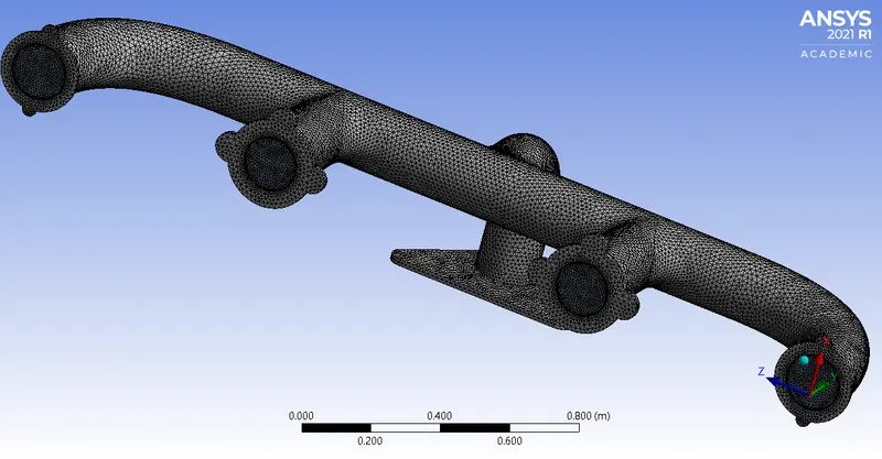
Fig.4.1. Exhaust Port Entire Mesh

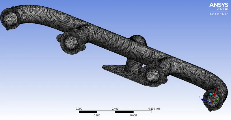
Fig.4.2. Exhaust Port – Solid Volume Mesh

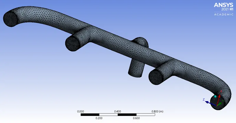
Fig.4.3. Exhaust Port – Fluid Volume Mesh

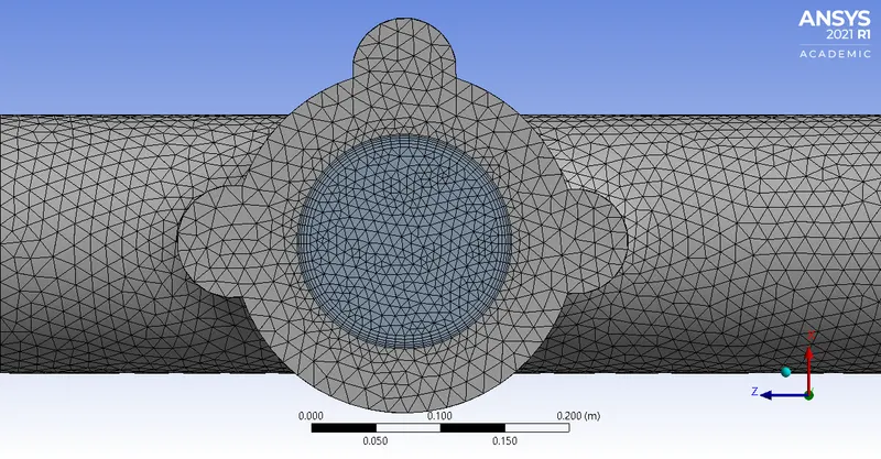
Fig.4.4. Exhaust Port - Inflation

5. MATERIAL PROPERTIES

Two different materials were chosen for the fluid and solid volume of the exhaust port.

Table 5.1: Solid Volume Material

PARAMETERS	SPECIFICATIONS
MATERIAL	ALUMINIUM
DENSITY	2719 kg/m3
SPECIFIC HEAT	871 J/kg-K
THERMAL CONDUCTIVITY	202.4 W/m-K

Table 5.2: Fluid Volume Material

PARAMETERS	SPECIFICATIONS
MATERIAL	AIR
DENSITY	1.225 kg/m3
VISCOSITY	1.7894×10-5 kg/m-s
THERMAL CONDUCTIVITY	0.0242 W/m-K
SPECIFIC HEAT	1006.43 J/kg-K

6. BOUNDARY CONDITIONS

Pressure – based steady solver using K-Ω SST and K-ε Realizable viscous model equations for the CHT analysis.

Table 6.1: Boundary Conditions

PARAMETERS	SPECIFICATIONS
THERMAL CONDITION	CONVECTION
INLET VELOCITY	5 m/s
INLET TEMPERATURE	700 K
OUTLET PRESSURE (GAUGE)	0 Pa
HEAT TRANSFER COEFFICIENT	20 W/m2-K
FREE STREAM TEMPERATURE	300 K

7. RESULTS

Under both viscous models, the contour plots of wall heat transfer coefficient, velocity, and velocity streamlines indicate that the heat transfer is higher around the bend near the outlet, as the velocity is highest. The maximum heat transfer coefficient at the wall obtained was -6.457e+3 W/m²-K and -6.392e+3 W/m²-K under K-ε and K-Ω viscous models respectively.

7.1. K-ε REALIZABLE

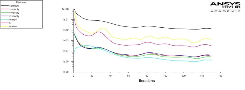
Fig.8.1.1. Graph of Scaled Residuals (K-ε)

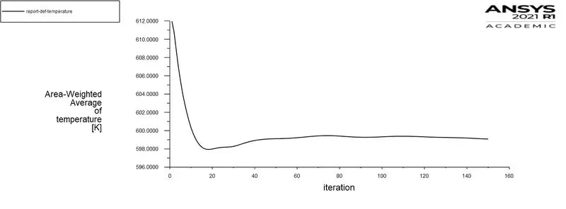
Fig.8.1.2. Graph of Area Weighted Average of Temperature (K-ε)

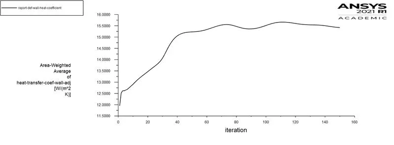
Fig.8.1.3. Graph of Area Weighted Average of Wall Heat Transfer Coefficient (K-ε)

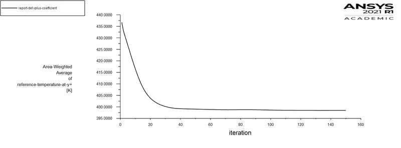
Fig.8.1.4. Graph of Area Weighted Average of Reference Temperature at Y+ (K-ε)

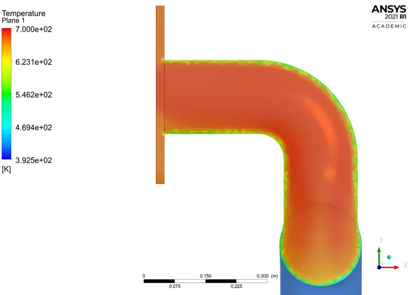
Fig.8.1.5. Contour of Temperature (K-ε)

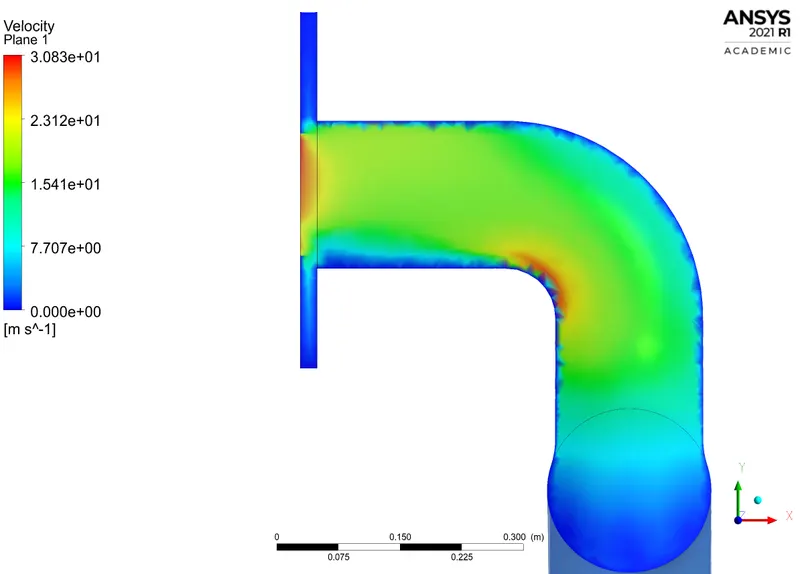
Fig.8.1.6. Contour of Velocity (K-ε)

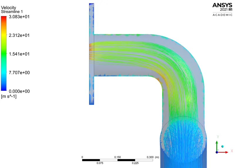
Fig.8.1.7. Contour of Velocity Streamlines (K-ε)

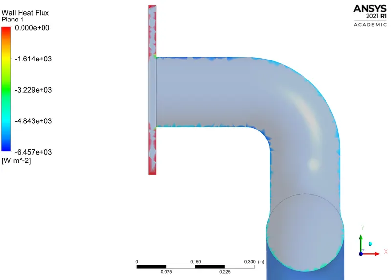
Fig.8.1.8. Contour of Wall Heat Transfer Coefficient (K-ε)

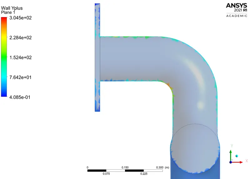
Fig.8.1.9. Contour of Reference Temperature at Y+ (K-ε)

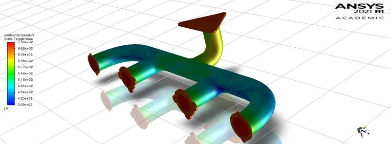
Fig.8.1.10. Entire Contour of Temperature (K-ε)

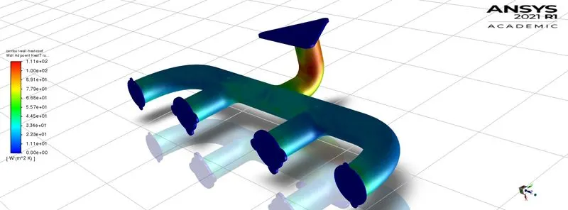
Fig.8.1.11. Entire Contour of Wall Heat Transfer Coefficient (K-ε)

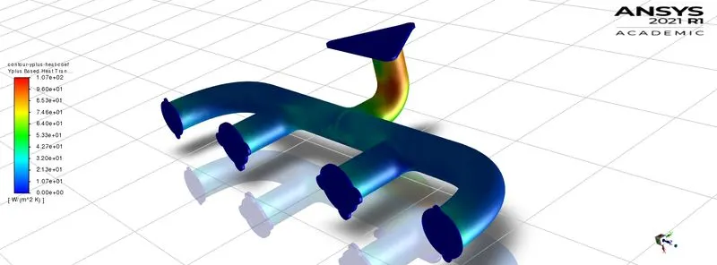
Fig.8.1.12. Entire Contour of Reference Heat Transfer Coefficient at Y+ (K-ε)

7.2. K-Ω SST

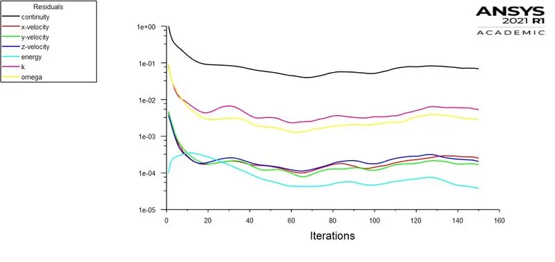
Fig.7.2.1. Graph of Scaled Residuals (K-Ω)

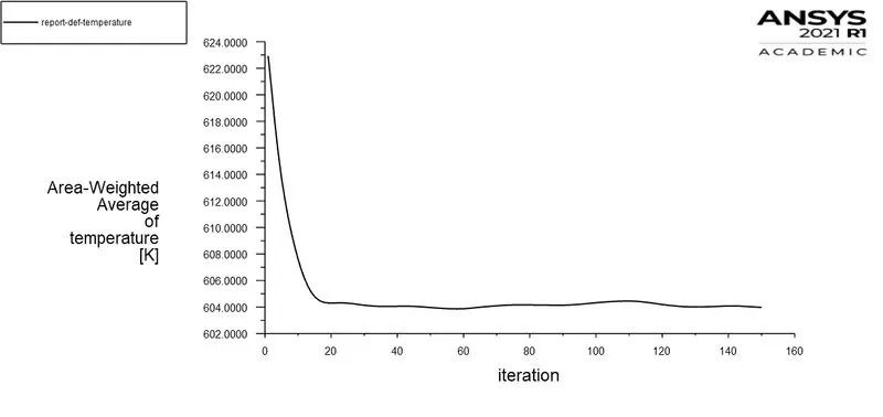
Fig.7.2.2. Graph of Area Weighted Average of Temperature (K-Ω)

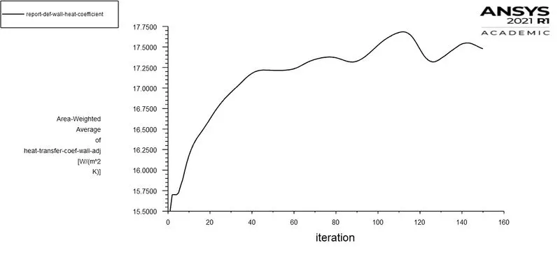
Fig.7.2.3. Graph of Area Weighted Average of Wall Heat Transfer Coefficient (K-Ω)

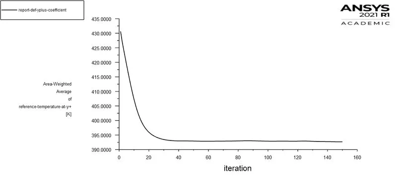
Fig.7.2.4. Graph of Area Weighted Average of Reference Temperature at Y+ (K-Ω)

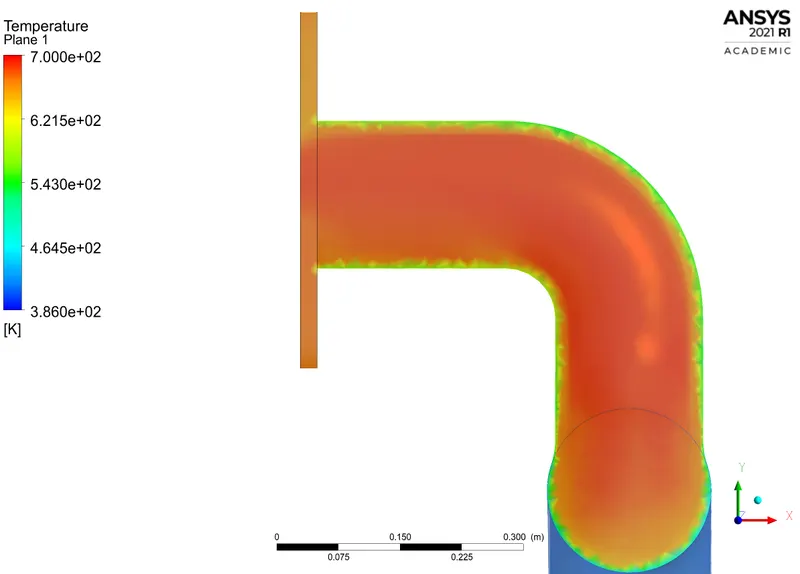
Fig.7.2.5. Contour of Temperature (K-Ω)

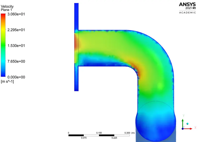
Fig.7.2.6. Contour of Velocity (K-Ω)

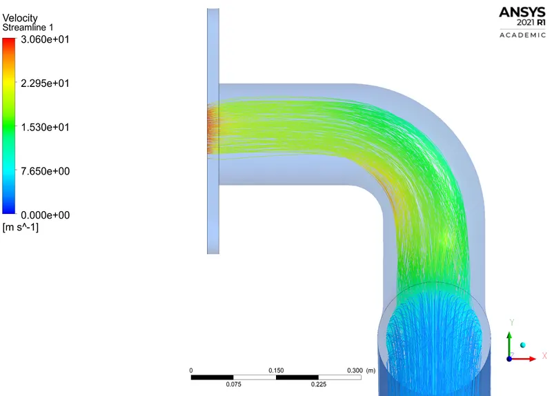
Fig.7.2.7. Contour of Velocity Streamlines (K-Ω)

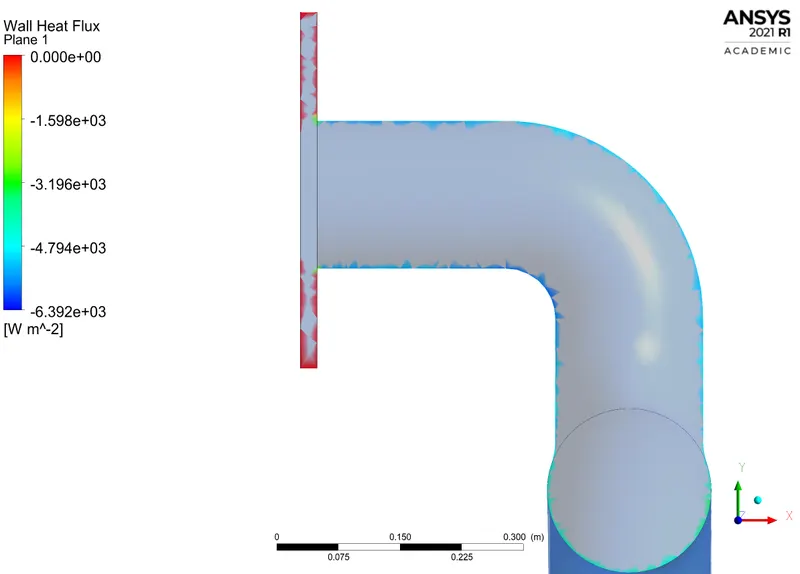
Fig.7.2.8. Contour of Wall Heat Transfer Coefficient (K-Ω)

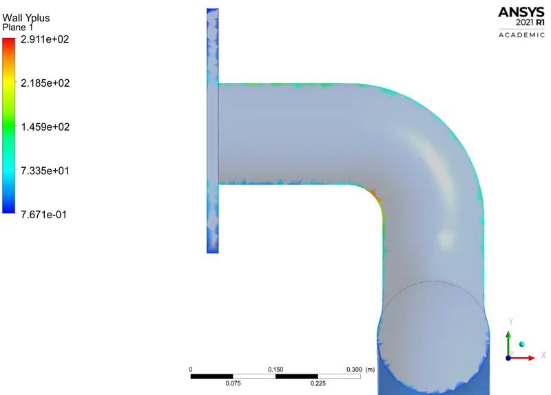
Fig.7.2.9. Contour of Reference Temperature at Y+ (K-Ω)

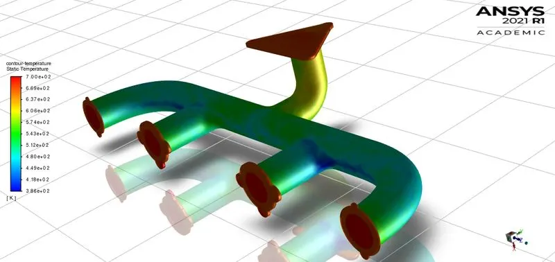
Fig.7.2.10. Entire Contour of Temperature (K-Ω)

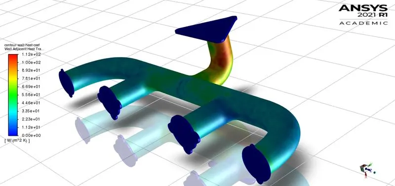
Fig.7.2.11. Entire Contour of Wall Heat Transfer Coefficient (K-Ω)

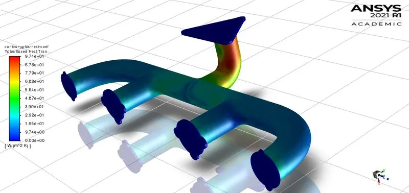
Fig.7.2.12. Entire Contour of Reference Heat Transfer Coefficient at Y+ (K-Ω)

8. CONCLUSION

• The highest heat transfer coefficient was attained where the velocity is highest.
• Highest wall and Y-based heat transfer coefficient contours obtained are near the outlet of the exhaust port, as predicted, due to higher mass flow.