Week 6.2 - Setting up a model (Hanging Node)

• AIM : To set up simulation problem for forced convection cooling.

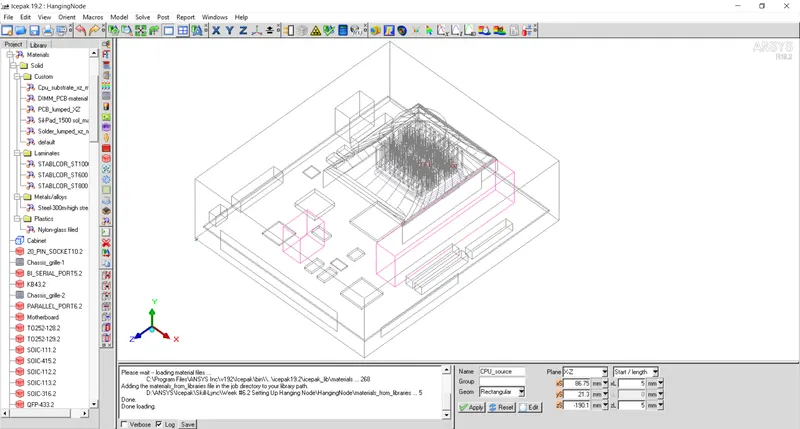
In order to maintain the temperature of the electronics components in the electronics enclosure under the maximum specified temperature, fans are used where the generation of heat is relatively high. The electronics model consists of CPU source generating `40W` of heat, a fan, a fan guide, a heat sink along with grills on the enclosure. Apart from the mentioned components, different components are mounted on the PCB that generates small amount of heat as show in figure below:

• Mesh Generation

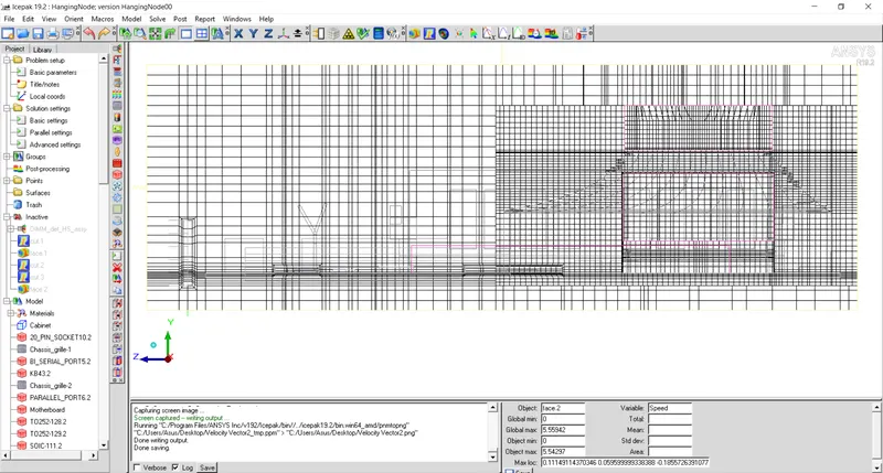
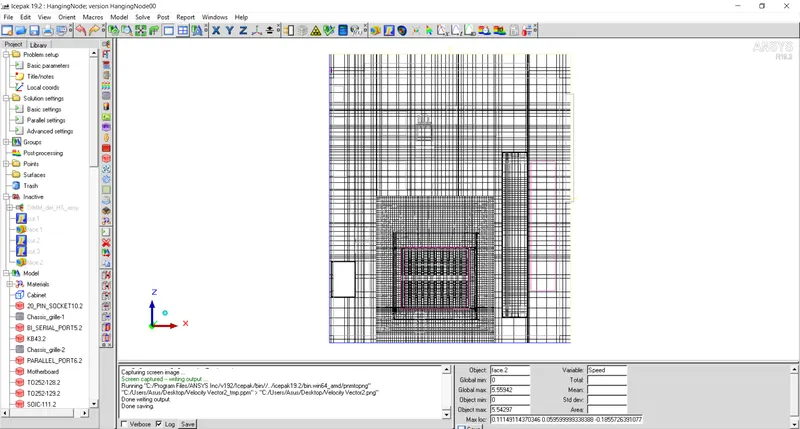
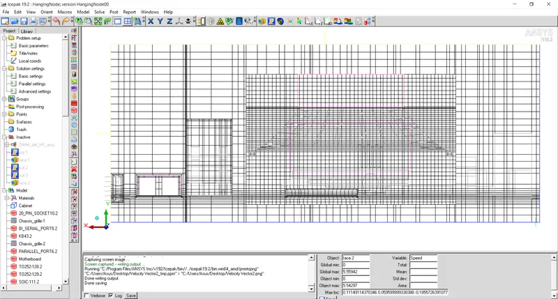
Non-conformal mesh has been generated to reduce number of cell counts. Also, to mesh complex CAD objects properly, multi-level meshing is used. Mesh details are shown below:

Mesh at mid X plane:

Mesh at mid Y plane:

Mesh at mid Z plane:

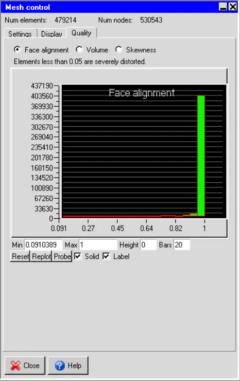
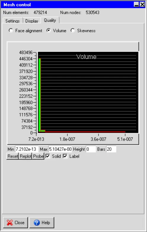
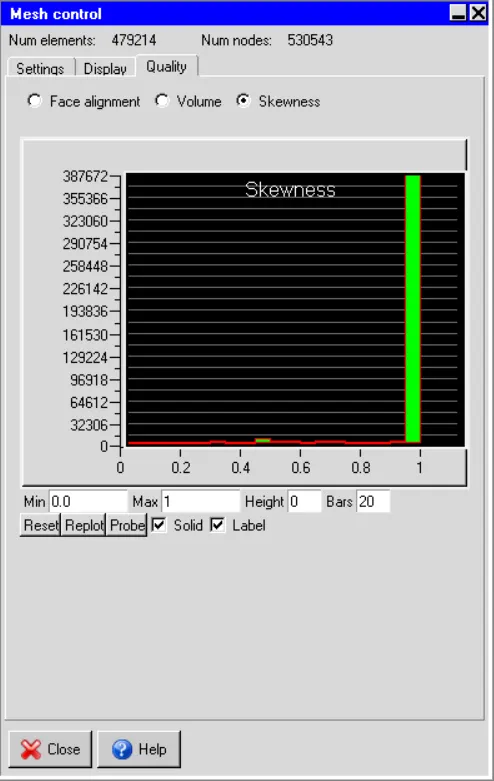
Mesh quality can be observed in the below figures.

Face alignment:

Volume:

Skewness:

After generating mesh and assigning appropriate parameters to the components, set up of model is an important step that defines the accuracy of the solution.

• Setting up model:

a. Basic Parameters

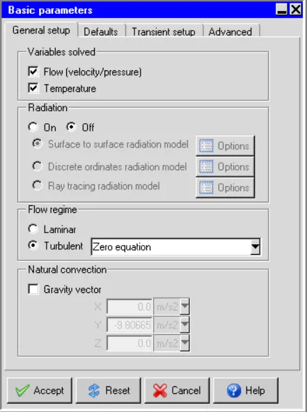
i. General setup:

In this problem, fan is used to maintain flow of air over the heat sink that will allow heat to be transferred from CPU source to the air. To solve the velocity and temperature within the domain, momentum and energy equation is solved. Hence, one has to select flow and temperature both as a solution variables.

As fan is used to maintain flow, major amount of heat will be transferred by forced convection. Radiation it turned off as it will be negligible.

Turbulent flow with zero equation is selected for solver.

Gravity is 'Off' as natural convection will be negligible.

ii. Defaults:

Ambient temperature is considered as `20^oC` with atmospheric pressure of `1atm`.

Material for fluid is `air` with default solid material as `Al-Extruded` and surface material as `Steel-Oxidised-surface`.

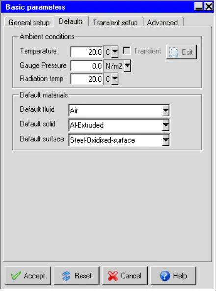
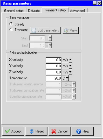
iii. Transient Setup:

In this solution, steady state condition is specified with initial temperature of `20^oC` inside entire domain and initial velocity of `0 m/s` in all the directions.

iv. Advanced:

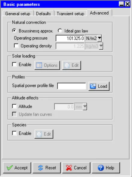
Default settings are kept as it is as natural convection will not have significant impact. By default Boussinesq approximation is used for natural convection flow.

As the enclosure is not subjected to external solar load, solar loading is kept Off.

If the enclosure is made to use for aviation industry, one has to consider altitude as it will affect density of air. Here in this case, it is assumed that enclosure is used on ground level.

Also, air only is consided as the fluid. If any other gases are involved along with air, mass fraction of different species can be specified by enabling Species.

Solution Setting:

i. Basic Settings

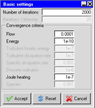
Number of iterations are set as 2000.

Convergence criteria are set as per the problem as shown below:

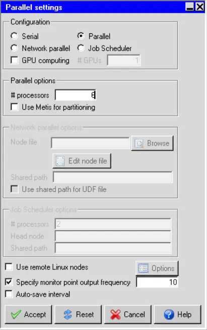
ii. Parallel Settings:

Parallel processing is used with #processor as 6.

iii. Advanced Settings:

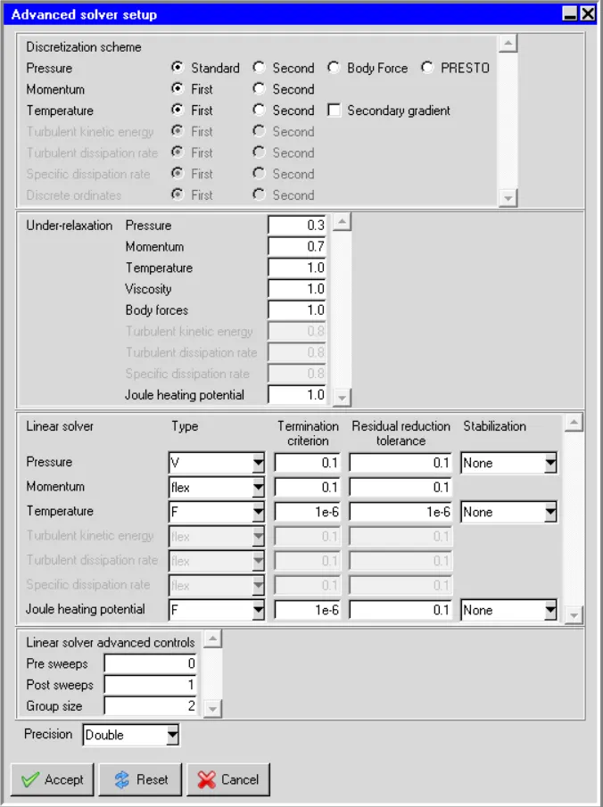
Standard discretization scheme is used for pressure along with first order descritization for momentum and temperature.

As the forced convection flow is there, under relexation factor of 0.3 and 0.7 are used for Pressure and momentum. For Temperature, Viscosity and Body forces default relaxation factor of 1 used.

As the problem does not contain natural convection and joule heating, no stablilization scheme is used.

Double precision is used to increase the accuracy of the solution.

Solve

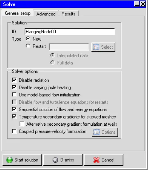
In this model, radiation is turned Off along with Joule heating is disabled.

Temperature secondary gradient for skewed meshes is turned On.

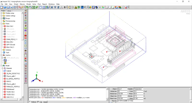
After setting up the simulation, monitor points are set at the four locations as shown in figure below.

• Convergence Plot

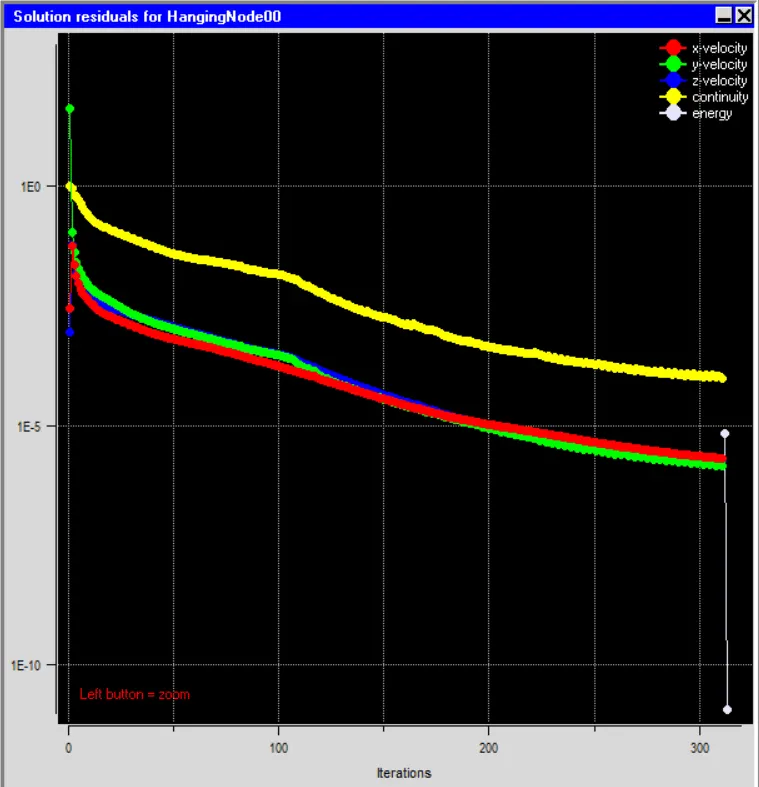
Residual plot for velocity (x, y and z), continuity and energy is shown below. It was observed that after 315 iterations.

• Results and Discussion

a. Temperature Contours

Temperature contour on the faces of the components is plotted in the figure shown below. It can be observed that maximum temperature of around `184^oC` is attained on the surface of DIMM_PCB. Also higher temperature is observed near the components generating heat.

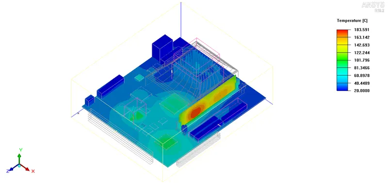
Temperature contour is also shown on the middle cut plane to observe variation of temperature in the domain for solid components as well as for air.

b. Velocity Contours

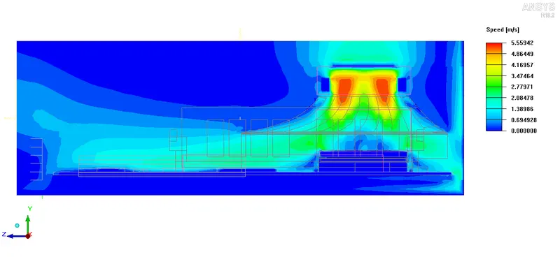
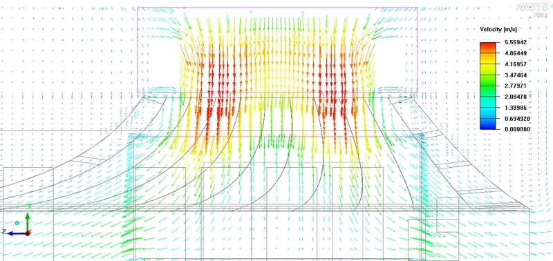
Velocity contour is plotted on the middle cut plane along the length of the enclosure to observe the velocity in the model. Maximum velocity is observed at the inlet of the fan. Maximum air speed observed is `5.6 m/s`.

c. Velocity Vector

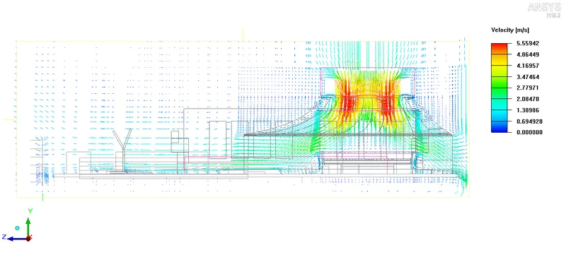
Velocity vector on the mid plane is shown in the figure below. Air velocity magnitude along with the direction of can be observed from the image. It can be observed that air is sucked by the fan and comes out from the fan with higher velocity in the downward direction.

• Conclusion

From the results it can be observed that maximum temperature of `184^oC` is observed where heat generation is taking place but the flow of air is not sufficient to carry away heat efficiently. The maximum temperature observed is above the acceptable limit for major electronics components, hence the design should be altered so that the maximum temperature should be within the limit. By limting the operating temperature of electronics componenets, one can increase life expentancy of components.