Week 6.1 - Setting up a model (Electronic enclosure)
AIM : To set up sover settings for simulation.
Steps to carry out simulation: 1. Geometry modeling,
2. Mesh generation,
3. Setting up simulation model,
4. Results and Discussion,
5. Conclusion.
1. Geometry Modeling
Geometry of the model is simplified in ANSYS spaceclaim. All the primitive shapes (cuboids, cylinders etc) are converted into ICEPAK objects using Level-0/1 simplification. Complex shapes such as enclosure is converted into ICEPAK compatible geometry using Level-3 simplification.
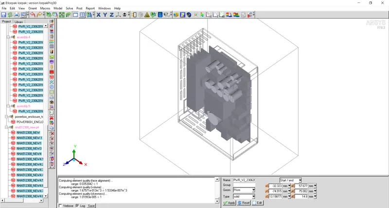
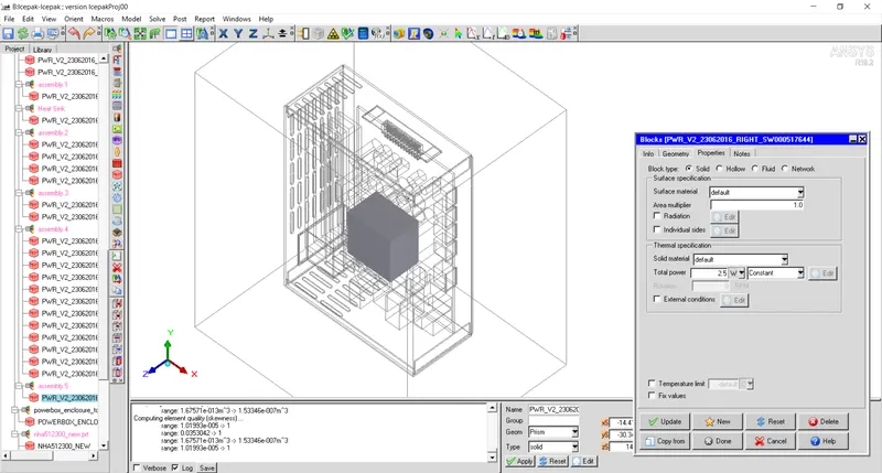
Power dissipation is assigned to different components as shown in the figures below:
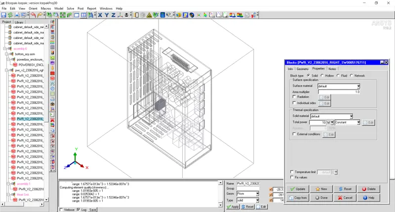
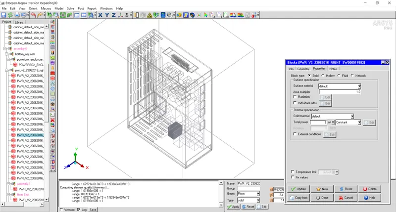
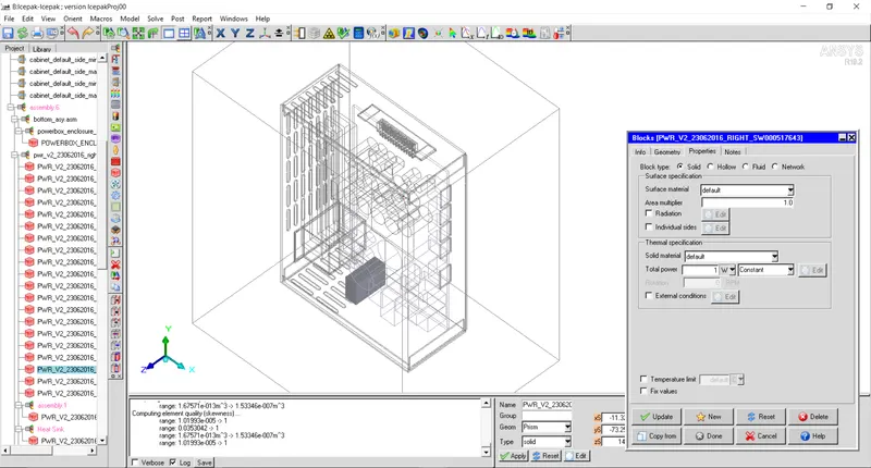
2. Mesh Generation
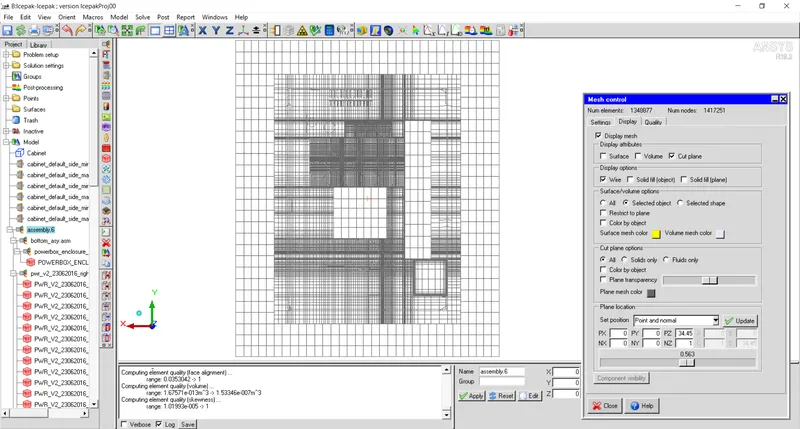
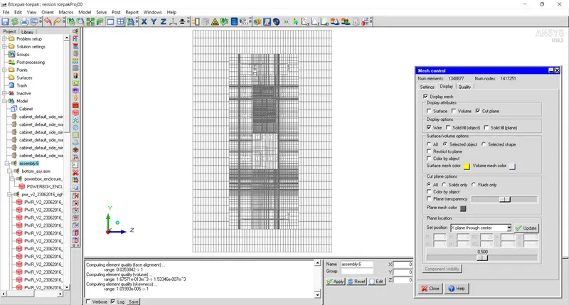
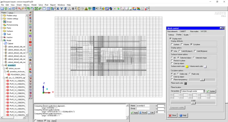
Non-conformal mesh is generated using 'seperate mesh assembly' to reduce the mesh count in the model. Multi-level meshing is used for enclosure because of complex shapes of opening in the enclosure.
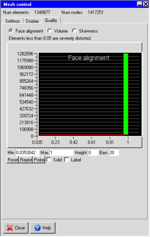
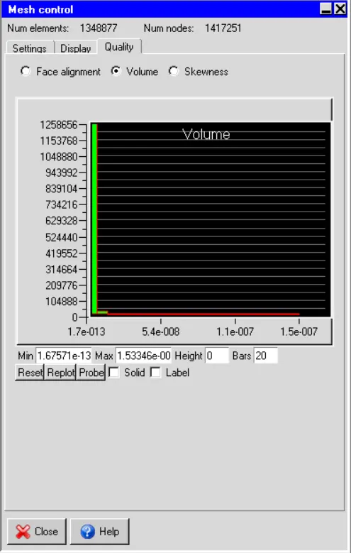
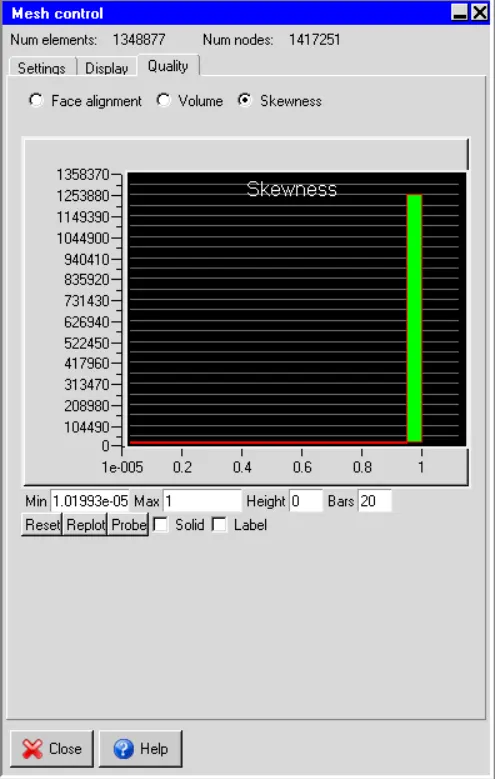
Mesh Quality
3. Setting up Simulation Model
Basic Parameters
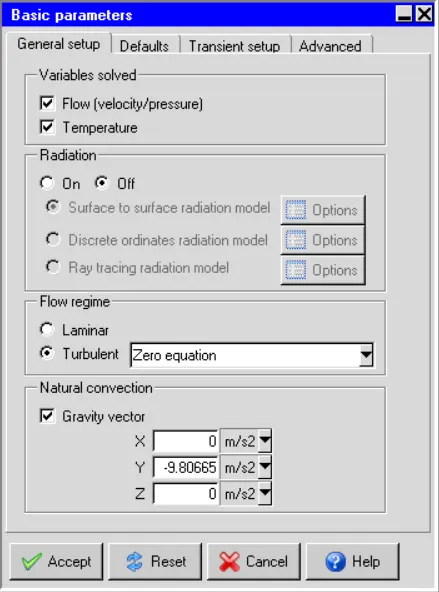
Temperature distribution and flow field is evaluated by solving Energy and Momentum equations respectively within entire domain of computation.
Radiation effect is neglected.
Zero equation model is used to solve turbulent phenomena in fluid domain.
Natural convection is turned on as heat trannsfer from the PCB components to the internal air and housing to the ambient air is by natural convection. As the air is heated its temperature increases and density decreases. Decrease in density will rise lighter fluid and velocity field is set up within the air domain. Gravity is enebled in -Y direction.
Ambient temperature considered is `20^oC` and pressure is `1 atm` is considered in fluid domain.
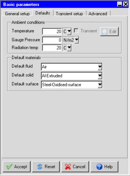
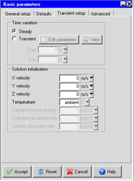
Steady state simulation is performed to evaluate temperature and velocity field. In steady state simulation iterations are performed for momentum and energy equations until the residual values reaches below specified number.
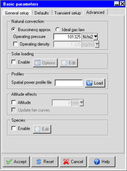
To take into effect of natural convection, density variation is approximated by Bousinessq approximation for air.
Soalr radiation on the enclosure surface is neglected and module is considered working at ground level.
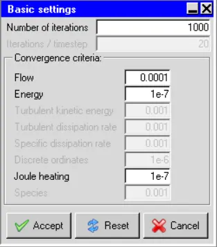
Basic Settings
Maximum number of iterations specified is 1000.
Residuals for velocity and temperature is specified as below.
Computation is performed until the iteration reaches maximum number or residual falls below spefified value.
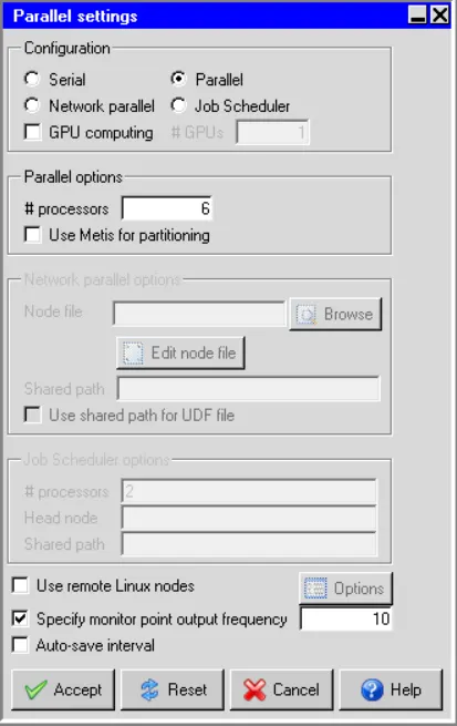
Parallel Setting
Parallel processing is used with 6 number of processors.
4. Results and Discussion
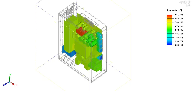
a. Temperature contour on face
Temperature contour is plotted on the face of all the components mounted on PCB. Surface temperature of all the PCB mounted components can be observed from the figure below. It is used to decide whether the component is safe under the specified operating parameters. Maximum temperature of `95^oC` is observed in the model.
b. Velocity vector on the mid plane
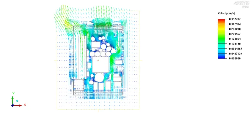
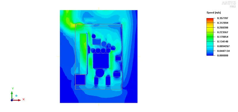
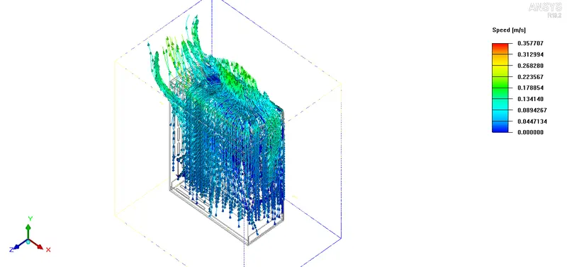
Velocity vector plot at the mid plane is shown in the figure below. It can be observed that air enters the enclosure from the bottom and side face openings, comes in contact with the heat dissipating components mounted on PCB. Air gets heated and comes out from the top openings. Maximum velocity of `0.35m/s` is attained because of natural convection.
c. Velocity contour on mid plane
d. Particle traces
5. Conclusion
Maximum face temperature of the components mounted on PCB is `95^oC` that is well below maximum specified temperatures for electronics components (around `125^oC`), hence the module is safe from thermal point of view.
Maximum velocity obtained is around`0.36m/s` as the flow is induced by natural convection. For forced convection cooling, higher magnitude of velocity is observed than that of natural convection.