Week 10 - MRF project
AIM : Apply MRF model for fan CAD model.
Why to use MRF model for fan?
Fan can be incorporated in the simulation using either fan objects available in Icepak or using CAD geometry of fan. When fan object is used in the model, it is not able to capture tangential and radial components of velocity and swirl as it does not take into account blade geometry and number of blades. Also, when active components are present in the vicinity of fan, it over predicts the flow physics that gives the lower temperature than it should be. To avoid the problems of fan object, one can used actual CAD geometry of fan and use MRF (Moving Reference Frame) model to accurately predict flow physics in the model and increase accuracy of the solution.
The procedure to carry out simulation with fan CAD geometry using MRF model is as follows:
a. Geometry Modeling
Unpack MRT_Tutorrial.tzr in ANSYS Icepak.
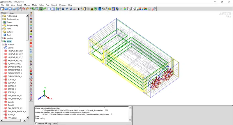
The model contains several PCBs mounted horizontally and vertically, power modules, fans, grills and other components mounted on PCB.
Create an assembly with name power module as shown below.
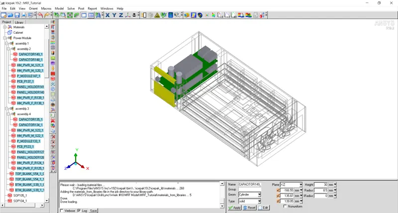
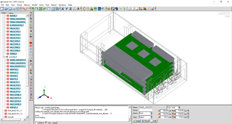
Create a nested assembly with four seperate assemblies as shown and name it as PCB assembly.
Create two fluid blocks for fan A and B.
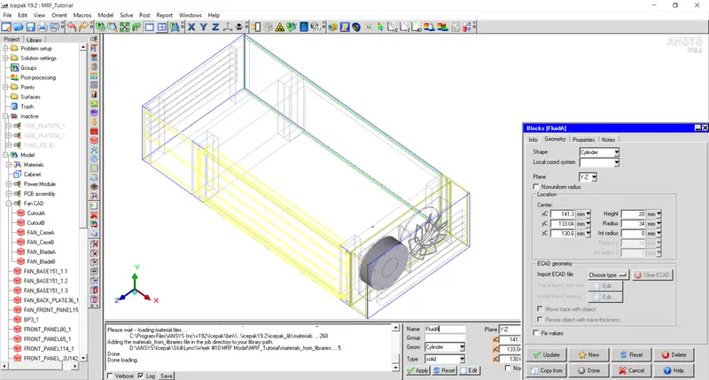
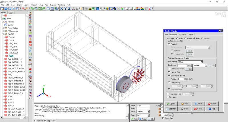
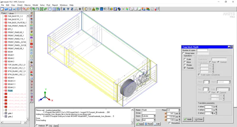
Create an assembly with name Fan CAD with following components.
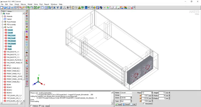
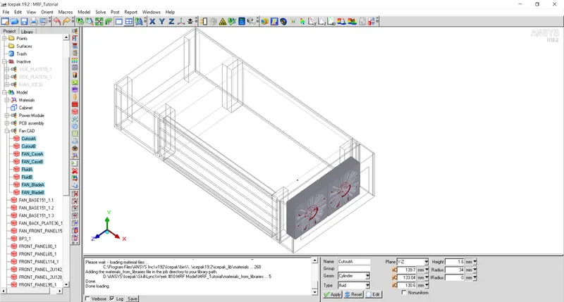
Specify meshing priority as Fan Blade > Fluid > Fan case > Cutout in Fan CAD assembly.
b. Boundary Conditions
All the two power module is given heat dissipation of 2W.
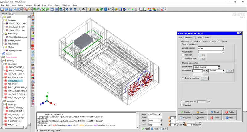
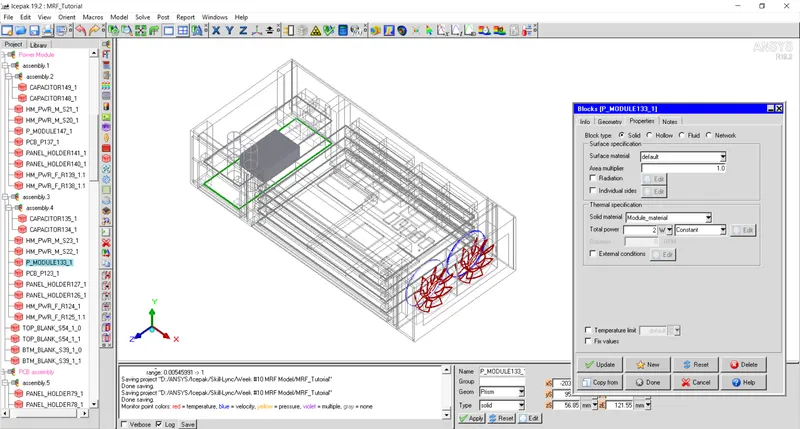
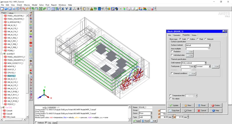
All the BGA is assigned with 3W of power dissipation.
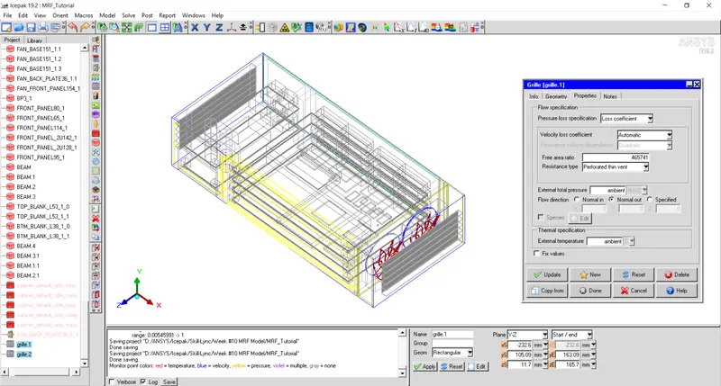
Both the grills is having free area ration of 0.465.
c. Monitor Points
Following monitor points are created for velocity and temperature.
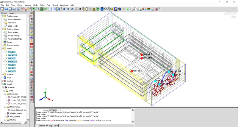
d. Mesh Details
Mesh seperately assemblies with appropriate slack values.
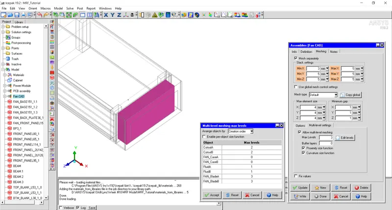
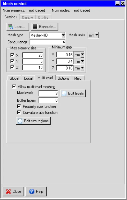
Generate mesh with following global mesh parameters.
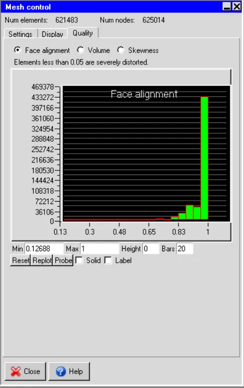
Mesh Quality
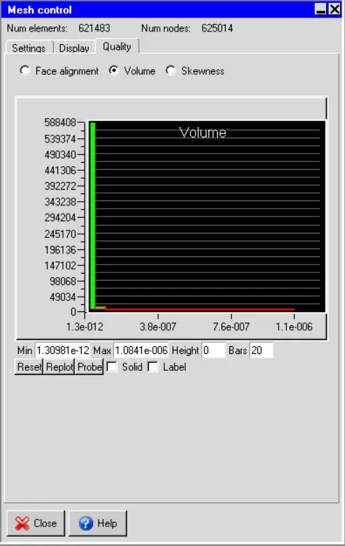
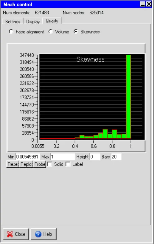
Visual inspection of mesh
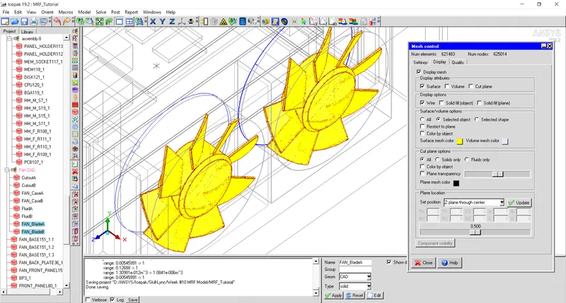
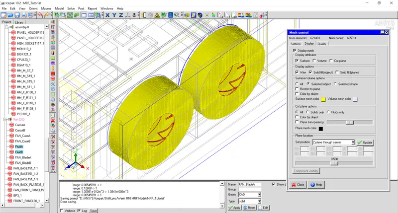
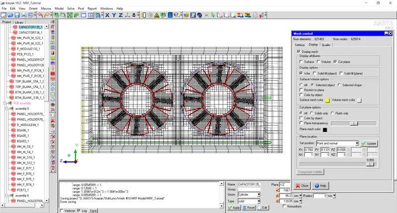
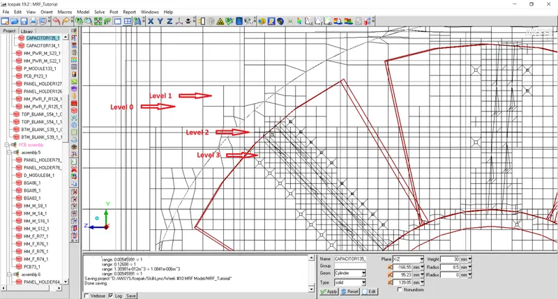
It can be observed that complex shapes such as fan blade, fluid domain etc are meshed properly that is very necessary for accurate solution of the model. From below cut plane multi-level mesh can be observed.
e. Solver Settings
Basic parameters
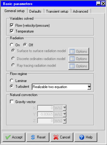
Use realizable two equations model to capture swirl properly when MRF model is used.
Flow and temperature field is solved within the model with radiation turned off.
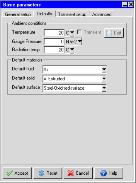
Default settings are kept as it is.
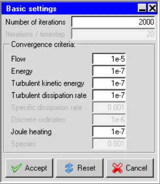
Basic settings
Set number of iteration as 2000 and lower the convergence criteria to have accurate results.
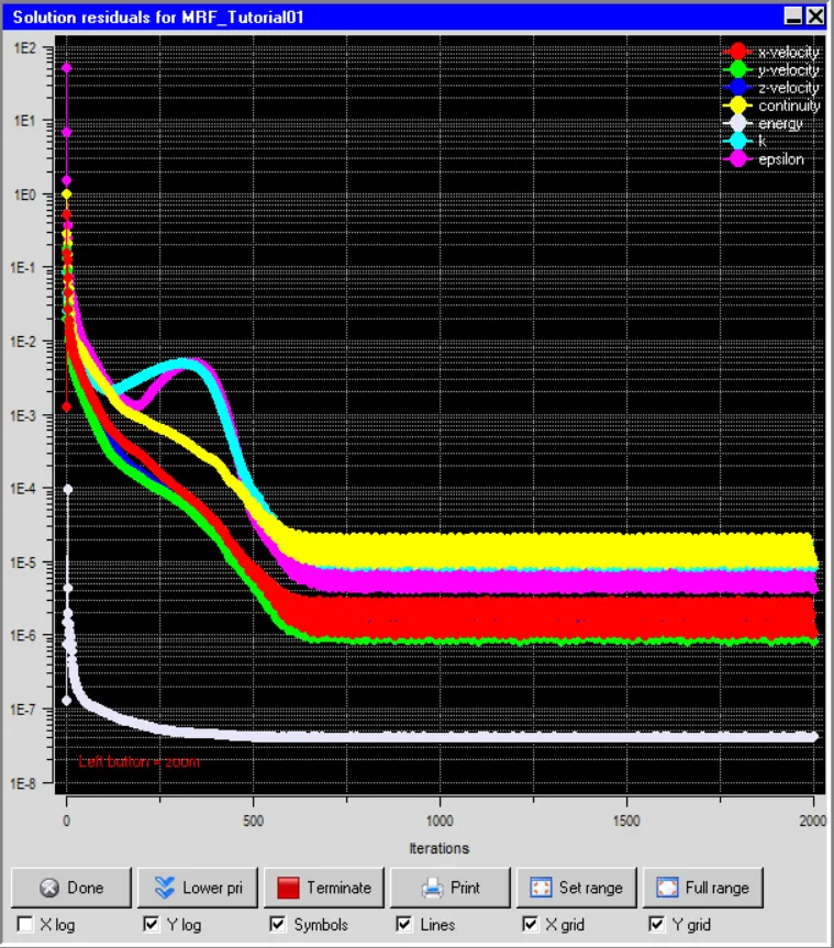
f. Convergence Plot
From convergence plot it can be seen that the residual values are below the specified criteria for entire domain after 600 iterations and hance steady state condition is achieved.
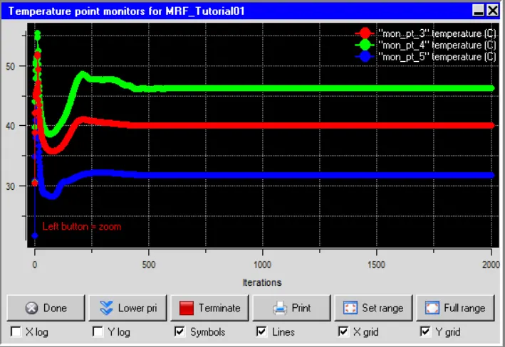
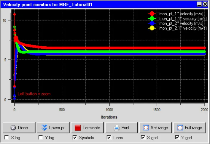
Monitor Plot
From both monitor plots it can be seen that temperature and velocity is constant at the respective locations with respect to the iterations and hence steady state condition is attained at those points.
g. Results and Discussions
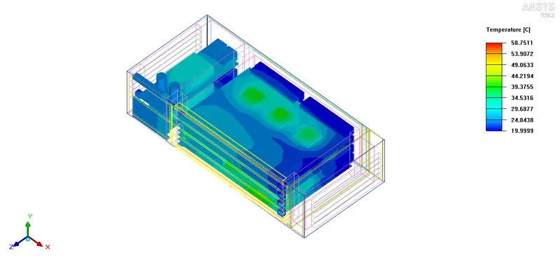
I. Temperature Contour on Component Faces
Temperature contour is plotted on the faces of all the components in the figure below. Maximum temperature of `58.75^oC` is observed in the model.
II. Velocity at the Mid Plane of Fan A
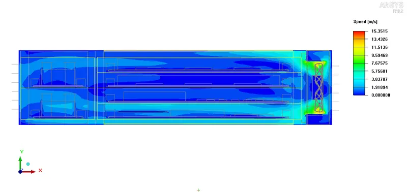
From the figure below it can be seen that higher velocity is observed at the periphery of fan because of centrifugal action and swirl generation. Maximum velocity of `15.35m/s` is observed near the fan.
III. Particle Streamlines from Fan
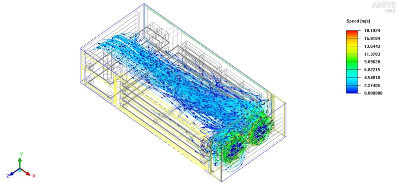
Particle trace is shown in the figure below. Swirl generated around the fan can be observed from the figure.
h. Conclusion
MRF model for fan CAD model is successfully implemented and maximum temperature of `58.75^oC` is observed that is in the safe limit for majority of the electronic components.
Swirl is generated and centrifugal spreading by the fan is observed in the model.