Week 5 - Curve fitting

1. What does popt and pcov mean? (Watch the video to get some context)

The curve_fit() function returns two items, which we call popt and pcov.

popt-

• The popt argument are the best-fit parameters (p optimal) for a and b.
• An array of optimal values for the parameters which minimizes the sum of squares of residuals.

pcov-

• The pcov variable contains the covariance matrix, which indicates the uncertainties and correlations between parameters.
• 2d array which contains the estimated covariance of popt. The diagonals provide the variance of the parameter estimate.

2. What does np.array(temperature) do?

np.array-

• to pass entire values of temperature.
• converts the python list of temperature to a numpy array since operations like pow are allowed on numpy arrays and not python lists.

3. What does the * in *popt mean?

• Helps to refer the values stored in the popt array.

4. Write code to fit a linear and cubic polynomial for the Cp data. Explain if your results are good or bad.

1. Program for linear curve fit.

import math
import matplotlib.pyplot as plt
import numpy as np
from scipy.optimize import curve_fit

# Curve fit function
def func(t,a,b):
    return a*t + b

# Reading thermodynamic data file
def read_file():
    temperature = []
    cp = []
    for line in open('data','r'):
        values = line.split(',')
        temperature.append(float(values[0]))
        cp.append(float(values[1]))

    return [temperature, cp]

# Main Program
temperature, cp = read_file()
popt, pcov = curve_fit(func, temperature, cp)
fit_cp = func(np.array(temperature), *popt)

plt.plot(temperature, cp,color="blue",linewidth=3)
plt.plot(temperature, fit_cp,color="red",linewidth=3)
plt.legend(['Actual data','Curve  fit'])
plt.xlabel('Temperature [K]')
plt.ylabel('Cp [J/Kg.K]')
plt.title('For linear curve')
plt.show()

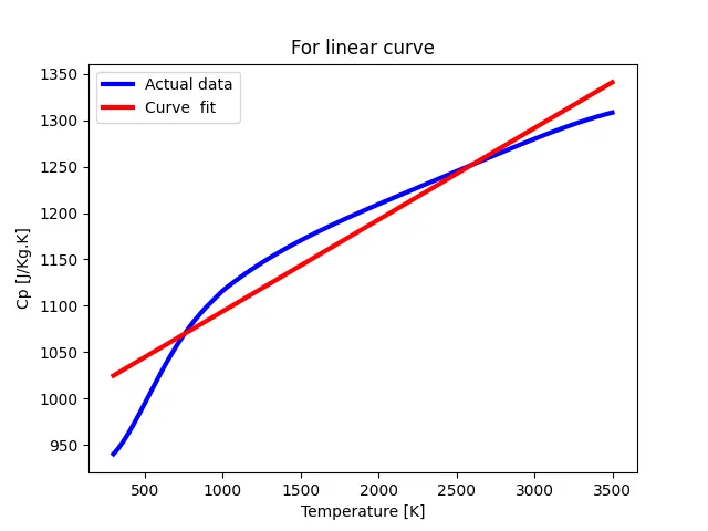
• Linear curve is not a fit curve.
• we can further increase the degree of curve to get a good fit to the actual curve.

2. Program for cubic polynomial curve fit.

import math
import matplotlib.pyplot as plt
import numpy as np
from scipy.optimize import curve_fit

# Curve fit function
def func(t,a,b,c,d):
    return a*pow(t,3) + b*pow(t,2)+ c*t + d

# Reading thermodynamic data file
def read_file():
    temperature = []
    cp = []
    for line in open('data','r'):
        values = line.split(',')
        temperature.append(float(values[0]))
        cp.append(float(values[1]))

    return [temperature, cp]

# Main Program
temperature, cp = read_file()
popt, pcov = curve_fit(func, temperature, cp)
fit_cp = func(np.array(temperature), *popt)

plt.plot(temperature, cp,color="blue",linewidth=3)
plt.plot(temperature, fit_cp,color="red",linewidth=3)
plt.legend(['Actual data','Curve  fit'])
plt.xlabel('Temperature [K]')
plt.ylabel('Cp [J/Kg.K]')
plt.title('For cubic polynomial curve')
plt.show()

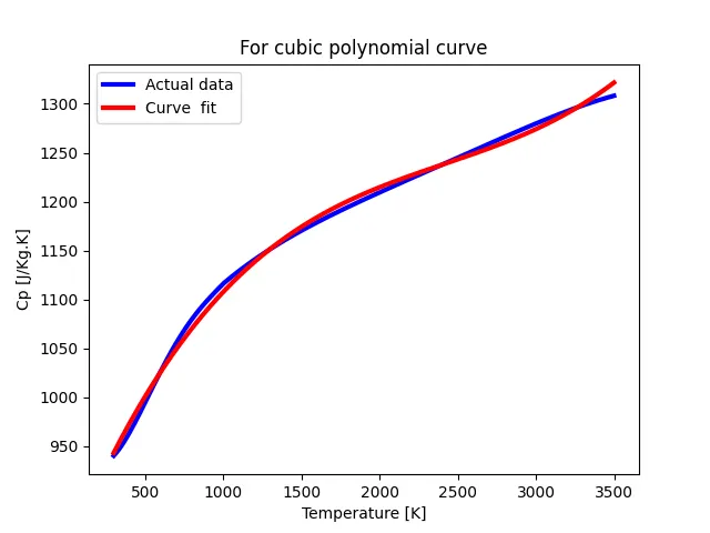
• Cubic curve is a good fit curve.
• But it is not a best fit or perfect fit curve.
• we can further increase the degree of curve to get a good fit to the actual curve.

5. What needs to be done in order to make the curve fit perfect?

• By increasing the degree of the curve we can make the perfect curve fit.
• If we further increase the degree of the curve to 9 then the curve will be the perfect fit curve.

Program for polynomial of degree 9 for curve fit.

import math
import matplotlib.pyplot as plt
import numpy as np
from scipy.optimize import curve_fit

# Curve fit function
def func(t,a,b,c,d,e,f,g,h,i,j):
    return a*pow(t,9)+b*pow(t,8)+c*pow(t,7)+d*pow(t,6)+e*pow(t,5)+f*pow(t,4)+g*pow(t,3)+h*pow(t,2)+i*t+j

# Reading thermodynamic data file
def read_file():
    temperature = []
    cp = []
    for line in open('data','r'):
        values = line.split(',')
        temperature.append(float(values[0]))
        cp.append(float(values[1]))

    return [temperature, cp]

# Main Program
temperature, cp = read_file()
popt, pcov = curve_fit(func, temperature, cp)
fit_cp = func(np.array(temperature), *popt)

plt.plot(temperature, cp,color="blue",linewidth=5)
plt.plot(temperature, fit_cp,color="red",linewidth=3)
plt.legend(['Actual data','Curve  fit'])
plt.xlabel('Temperature [K]')
plt.ylabel('Cp [J/Kg.K]')
plt.title('For polynomial curve of power 9')
plt.show()

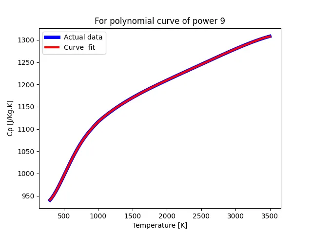
6. Show empirically as to how well your curve has been fit.

• By increasing the degree of the curve we can make the perfect curve fit.
• we can make best fit by further increasing degree of the curve.
• I further increased the degree of the curve to 9 then the curve is the perfect fit to actual curve.
• we can also use optmising method to get best or perfect fit to the actual one.