Week-4 Challenge WOT Condition Part-2
Aim: To understand the basics of Powertrain Blockset.
Objective:
- To write what is the difference between the mapped and dynamic model of engine, motor and generator? How the model type can be changed?
- To describe how does the model calculate miles per gallon? and which factors are considered to model fuel flow?
- To run the HEV ReferenceApplication with WOT drive cycle. Change the grade and wind velocity in the environment block. Comment on the results.
- To compare the simulated results of hybrid and pure electric powertrains, keeping all other parameters same.
Powertrain Blockset
Powertrain Blockset provides fully assembled reference application models of automotive powertrains, including gasoline, diesel, hybrid, and electric systems. It includes a component library for simulating engine subsystems, transmission assemblies, traction motors, battery packs, and controller models. Powertrain Blockset also includes a dynamometer model for virtual testing. MDF file support provides a standards-based interface to calibration tools for data import.
Powertrain Blockset provides a standard model architecture that can be reused throughout the development process. We can use it for design tradeoff analysis and component sizing, control parameter optimization, and hardware-in-the-loop testing. We can customize models by parameterizing components in a reference application with our data or by replacing a subsystem with our model.
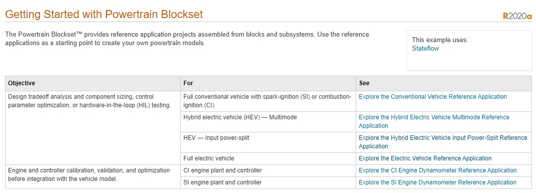
To model a powertrain system for our project, we can select a reference application based on the powertrain type. Each reference application includes plant models, controllers, a longitudinal driver, and drive cycle data.
The reference applications come with a Simulink Projects configuration. Simulink Projects enables management and version control for top-level model files, component model files, and scripts.
Reference applications serve as a starting point for our system model. To tailor a reference application to our powertrain project, parameterize the components in the reference application using data from a domain-specific tool, a test bench, or a vehicle. Depending on our application and powertrain configuration, we might need to select the type of component models and further customize the system model.
The component library in Powertrain Blockset provides blocks of physical systems and controllers for:
- Propulsion
- Transmission
- Drivetrain
- Energy storage
- Longitudinal vehicle dynamics
- Drive cycle data and longitudinal driver
All the models in Powertrain Blockset, including the reference applications and components in the library, are fully open for customization. We can use Simulink Projects to manage model variants including variant selection, version management, and comparison.
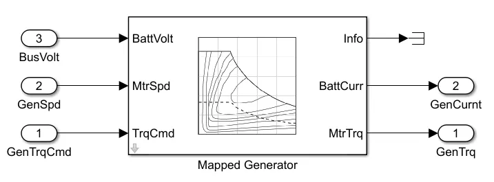
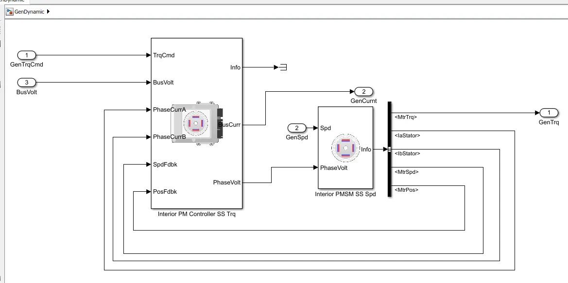
Powertrain Blockset provides two types of combustion engine models: mapped and dynamic. Mapped engines represent macro engine behaviour as a set of lookup tables (brake torque, fuel flow, air mass flow, exhaust temperature, efficiency, and emissions) as functions of commanded load and measured engine speed. Dynamic engines decompose engine behaviour into individual component models that account for engine dynamics, most notably intake airflow and turbocharger dynamics.
We can switch between engine model types based on your application. Dynamic engine models are suitable for designing control, estimator, and diagnostic algorithms that depend on dynamic subsystem states, for example, in closed-loop AFR control algorithm development. Mapped engine models are suitable for analysis and design activities that do not require engine subsystem dynamic characteristics, for example, in engine and transmission powertrain matching analysis for fuel economy, emissions, and performance tradeoffs.
Both the SI and CI engine models run in real-time for hardware-in-the-loop (HIL) testing.
Q1. a) What is the difference between the mapped and dynamic model of engine, motor and generator?
|
Mapped
|
Dynamic
|
Mapped Model for Electric Motor
Dynamic Model for Electric Motor
Q1. b) How can you change the model type?
We can switch between mapped and dynamic model types based on the application:
- Open the powertrain module blocks for the required vehicle.
- Click on passenger car/vehicle block and select an electric plant or engine.
- Right-click on Engine/EV motor/generator based on the vehicle model and select subsystem & model reference.
- In subsystem & model reference selecting option convert to the variant subsystem.
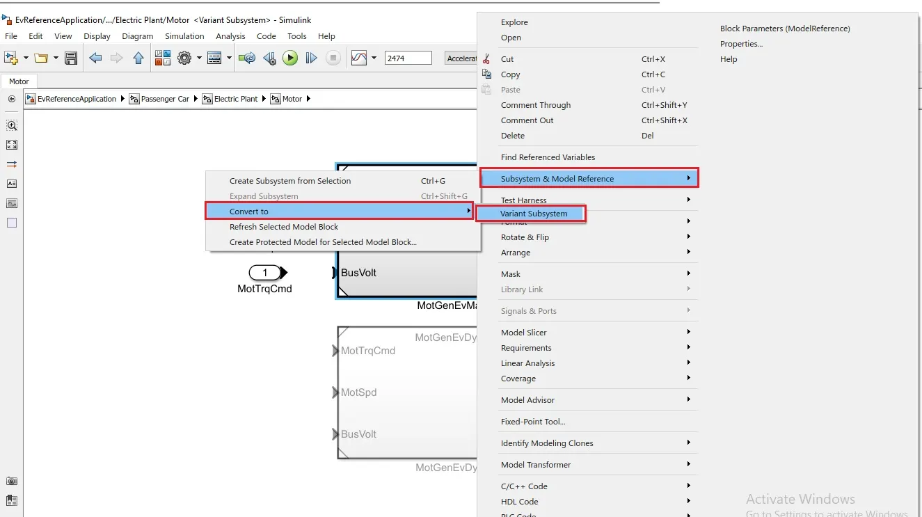
- Then by using model explorer
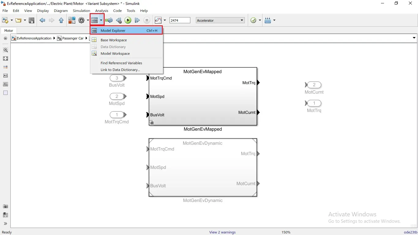
- The model type can be changed as shown in the below image.
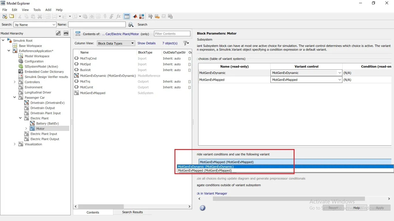
Q2. a) How does the model calculate miles per gallon?
Miles per Gallon: Miles per gallon (MPG) is a fuel economy rating determined by how far a car can travel using one gallon of gasoline or diesel for a conventional IC Engine vehicle. In the case of an electric vehicle, this is a measure of how much electrical energy is consumed by the battery pack to travel a fixed distance.
Per gallon of gasoline-equivalent for electric cars:
Burning one gallon of gas produces 121.3MJ. To generate the same amount of heat by way of electricity, it takes 33.7 kilowatt-hours (kWh). So if an electric vehicle can travel 100 miles on 33.7 kWh of electricity, then we can rate it at as 100 MPGe.
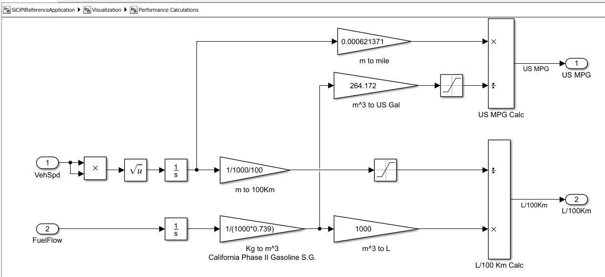
The power train block set has a model that calculates the miles per gallon for all kinds of vehicles.
1. For Conventional Vehicle
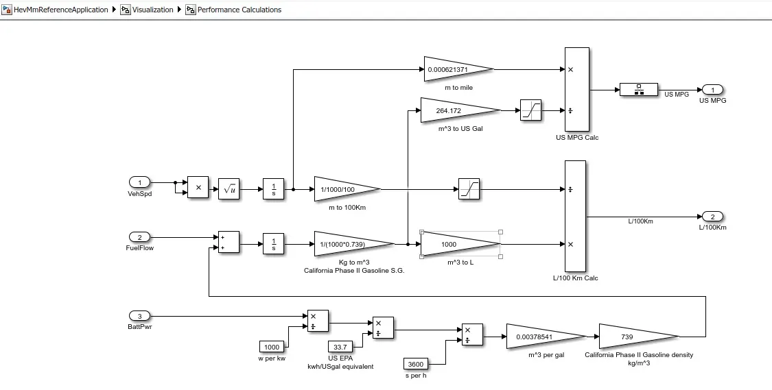
2. For hybrid electric vehicles-
3. For electric vehicles-
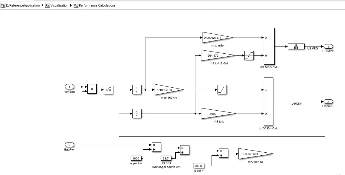
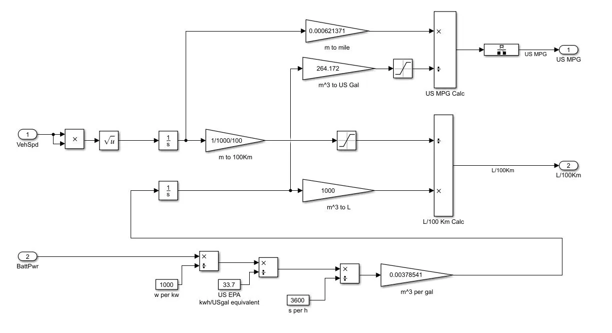
The model takes an input of vehicle speed, fuel flow and battery power to calculate fuel consumption and the equivalent battery consumption to calculate the miles per gallon.
Vehicle speed & Fuel flow:
- Vehicle speed is an important factor while considering the fuel consumption at that particular time, to determine fuel consumption throughout the drive cycle.
- To convert speed to Distance, Integrate speed with time doing the same of converting the velocity to get the distance covered by integrating.
- Then the Fuel flow is expressed as the mass flow rate (i.e) the amount of fuel at each moment in kg/Sec. Now integrating this will result in the mass of the fuel and by using this 1/(1000*0.739) we convert it to the volume and multiply by 1000 to get it in Litres.
- By comparing the two results we can get the amount of litre consumed to Run for 100km.
Battery Power:
- The amount of energy from battery power required to propel the vehicle Equivalent to that of the Engine is calculated here.
- The battery power is given in Watts and it is converted to kW by dividing with 1000.
- Then converting the Energy from kWh to equivalent energy in US gallon of automotive gasoline by dividing with 33.7. since we get the energy in US Gallons equal in kWh, to get the energy of equivalent US Gallons per seconds dividing with 3600 and we convert the hour to seconds.
- Then multiplying with 0.00378541 converting the US Gallons per sec to the volume of the fuel flow in (`m^3/s`) and then we multiply with 739 (California Phase II Gasoline density) (i.e) `m^3/s times (kg)/m^3` which gives the result as mass flow rate kg/s.
- Then finally the Battery energy equivalent in kg/s is given as an input for the fuel flow parameter to find the equivalent US Gallons energy and estimate the Miles per Gallons.
Calculating Miles per Gallon:
- The inputs from the vehicle speed (i.e) the Distance we found (in meters) are taken into the calculation and it is converted to the miles by multiplying with 0.000621371.
- Then the inputs from fuel flow (Battery energy + Fuel energy) taken in m^3 and are converted into equivalent US Gallons by multiplying with 264.172.
- Then the two inputs Miles covered and equivalent US Gallon are further divided and the result is got in Miles / Gallon.
Q2. b)Which factors are considered to model fuel flow?
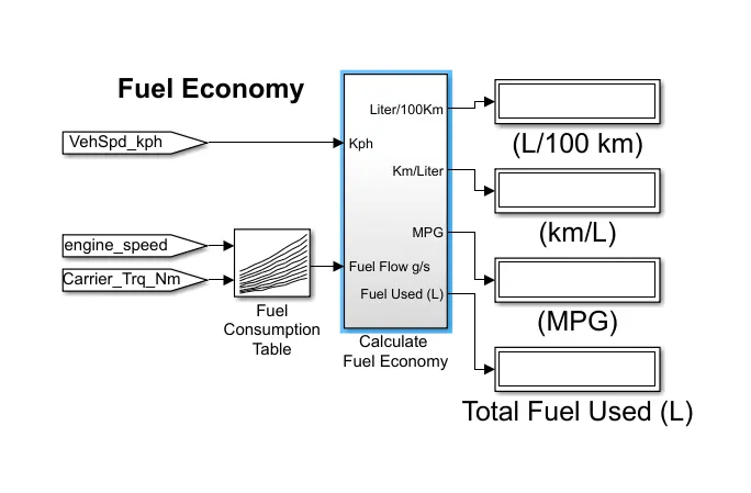
Factors considered in the model fuel flow are Fuel Economy and Fuel Consumption:
1. Fuel Economy:
The fuel economy of an automobile relates distance travelled by a vehicle and the amount of fuel consumed. Consumption can be expressed in terms of volume of fuel to travel a distance, or the distance travelled per unit volume of fuel consumed. Since fuel consumption of vehicles is a significant factor in air pollution, and since the importation of motor fuel can be a large part of a nation's foreign trade, many countries impose requirements for fuel economy. Different methods are used to approximate the actual performance of the vehicle. The energy in the fuel is required to overcome various losses (wind resistance, tire drag, and others) encountered while propelling the vehicle, and in providing power to vehicle systems such as ignition or air conditioning. Various strategies can be employed to reduce losses at each of the conversions between the chemical energy in the fuel and the kinetic energy of the vehicle. Driver behaviour can affect fuel economy; manoeuvres such as sudden acceleration and heavy braking waste energy. However electric cars do not directly burn fuel, and so do not have fuel economy per se, but equivalence measures.
Major Factors Considered in the Fuel Economy:
Vehicle speed
Engine speed
Motor torque
2. Fuel Consumption:
Fuel consumption is the inverse of fuel economy. It is the amount of fuel consumed in driving a given distance.
Q3. a) Run the HEV ReferenceApplication with WOT drive cycle.
Hybrid Electric Vehicle:
A hybrid electric vehicle (HEV) is a type of hybrid vehicle that combines a conventional internal combustion engine (ICE) system with an electric propulsion system hybrid vehicle drivetrain. The presence of the electric powertrain is intended to achieve either better fuel economy than a conventional vehicle or better performance. There is a variety of HEV types and the degree to which each function as an electric vehicle (EV) also varies. The most common form of HEV is the hybrid electric car, although hybrid electric trucks (pickups and tractors) and buses also exist.
Architecture:
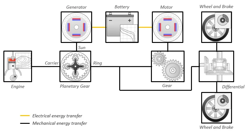
In MATLAB using Powertrain Blockset - Design tradeoff analysis and component sizing, control parameter optimization, or hardware-in-the-loop (HIL) testing for HEV-Input Power Split under that exploring Hybrid Electric Vehicle Input Power-Split Reference Application.
Selecting - autoblkhevIpsStart
Simulation Model: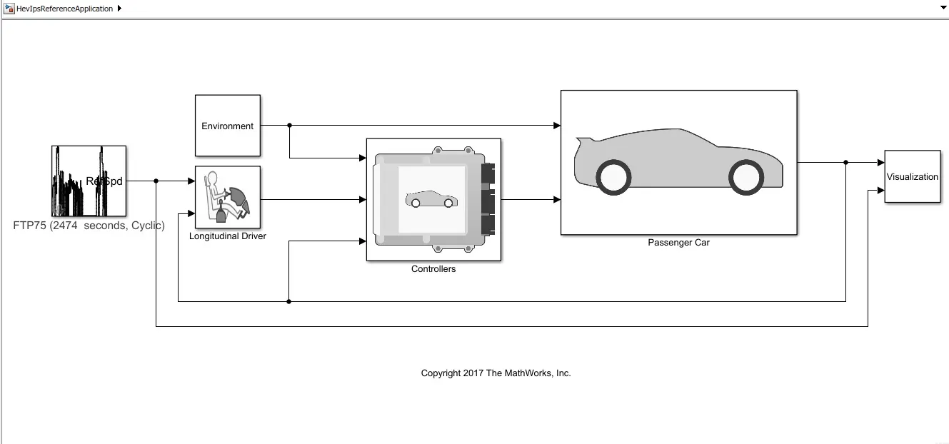
Case I:
For the first block selecting the input drive cycle i.e Wide Open Throttle(WOT), keeping grade as 0 and wind velocity as 0 and other parameters as default.
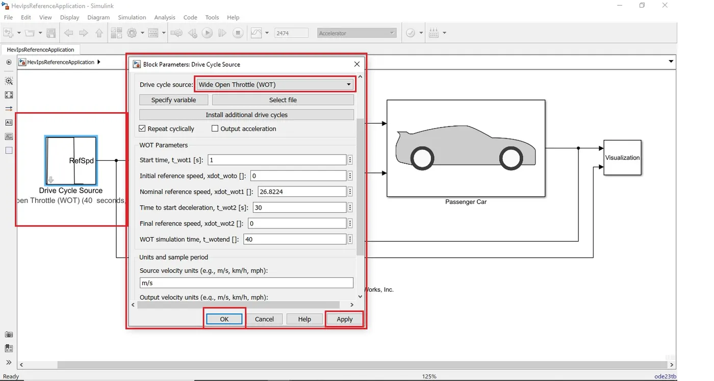
The simulation is done for Hybrid electric vehicle with Wide open Throttle Drive cycle.
The Total cycle time = 60 seconds
Time to start deceleration = 30seconds
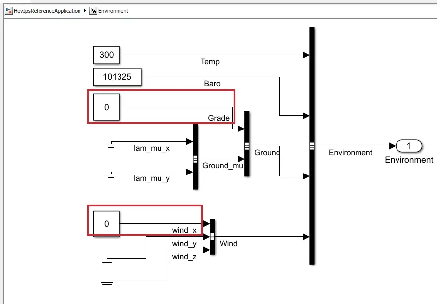
The Grade angle = 0 degree
The wind velocity = 0 m/s
Results:
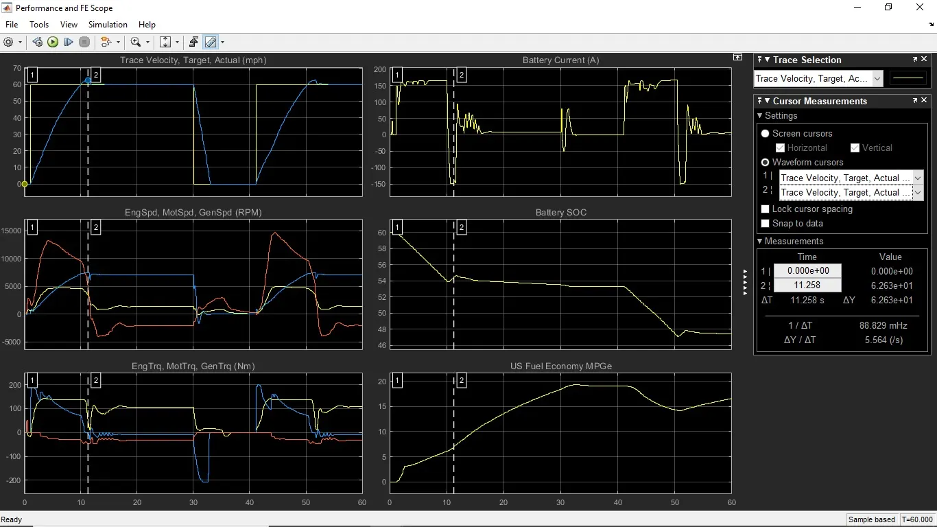
The above image shows the results for the simulation and it consists of six different plots.
Cursor measurement helps in reading results in a better way. The cursor enables us to study the behaviour of other result parameters corresponding to the acceleration of the vehicle.
Plot 1: Trace Velocity, Target, Actual(mph)
It shows the velocity of the vehicle for the Drive cycle data with the Time scale on the x-axis.
Traced velocity is given as input command & actual velocity is output. The actual graph doesn’t match with input traced velocity due to limited instantaneous current/power available.
The top speed achieved = 63 mph
The acceleration time to reach 63 mph = 11.258 seconds
The deceleration time from 60 to minimum = 3.164 seconds
From the plot, it can be stated that the top vehicle speed achieved very fast i.e within 11 seconds the same speed remains up to 30 seconds. Top speed reach to minimum speed in just 3.16 seconds. Similarly, the cycle continues, the drive Cycle is of 40 seconds and simulation is ran for 60 seconds for a proper conclusion.
Plot 2: Engine Speed, Motor Speed, Generator Speed(RPM)
It shows the changes in the speed of the engine, motor and generator in rpm throughout the drive cycle.
Peak Engine speed = 4787 Rpm
Peak Motor speed = 7437 Rpm
Peak Generator speed = 14610 Rpm
The engine, motor, generator speed is increasing when the vehicle speed is increasing. It can be seen that generators & engine speed have reached the peak values when battery SOC started falling after 40 seconds.
The motor initiates the initial acceleration and is capable to produce enough propulsion power to reach the specified maximum velocity. However, the motor is activated as soon as the maximum velocity is achieved indicating that a combined effort is required to maintain the velocity. The engine continues to operate which in turn is the input for the generator for producing electricity to reach the default SOC as specified in the control strategy.
Plot 3: Engine Torque, Motor Torque, Generator Torque(Nm)
It shows the torque characteristics and its changes of engine, motor and generator in (Nm) throughout the drive cycle.
Peak Engine torque = 143 Nm
Peak Motor torque = 200 Nm
Peak Generator torque = 51 Nm
With Wide-open throttle specification, the motor runs at maximum torque, however, the power distribution stabilizes between the motor and the engine as the vehicle reaches the desired velocity. A negative value for the generator indicates the engine torque is used to charge the battery as well during the propulsion time.
Plot 4: Battery Current (A)
It shows the battery current values (A) and its changes for various acceleration inputs as per the Drive cycle.
The peak current discharge from the battery = 164.63 A
The peak current charging to the battery = -147.68 A
With Wide-open throttle specification, the powertrain draws maximum current from the battery and stabilizes as the conditions are met and the engine is activated. A negative battery current value indicates regenerative braking and charging by the engine.
Plot 5: Battery SOC
It shows the battery state of charge SOC (%) and its changes corresponding to the driving inputs.
The state of charge decreased from 60% to 47.4% of charge in 60 seconds, for the specified driving conditions.
Plot 6: US Fuel economy MPGe
Shows the Fuel Economy as Mile per Gallons for the corresponding input driving conditions.
According to the drive cycle, the vehicle achieved its maximum speed at 11th second and the speed is constant up to 30th second of drive cycle (from plot 1), so it can be observed (from the plot) that fuel requirement is also increasing with the increase in speed till the speed is constant. After this constant speed vehicle speed is decreasing and the vehicle is at lowest speed for next 10-12 seconds and during this, the fuel requirement is also decreasing, and the same drive cycle and fuel requirement is repeated.
Q3. b)Change the grade and wind velocity in the environment block. Comment on the results.
Simulink Model:
Case II:
For the first block keeping the input drive cycle i.e Wide Open Throttle(WOT) same as used earlier, Changing the grade and wind velocity, keeping all other parameters as default.
The simulation is done for Hybrid electric vehicle with Wide open Throttle Drive cycle.
The Total cycle time = 60 seconds
Time to start deceleration = 30seconds
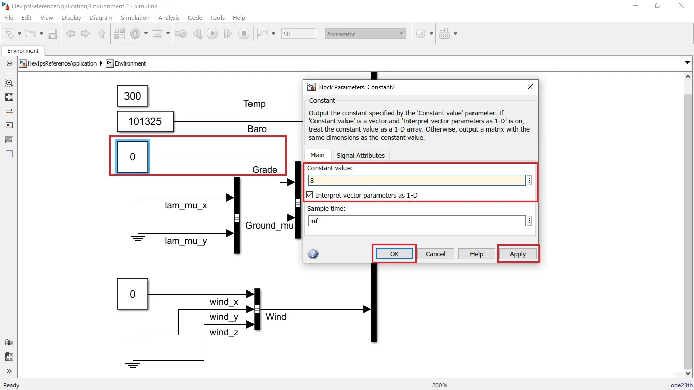
The Grade angle = 8 Degrees
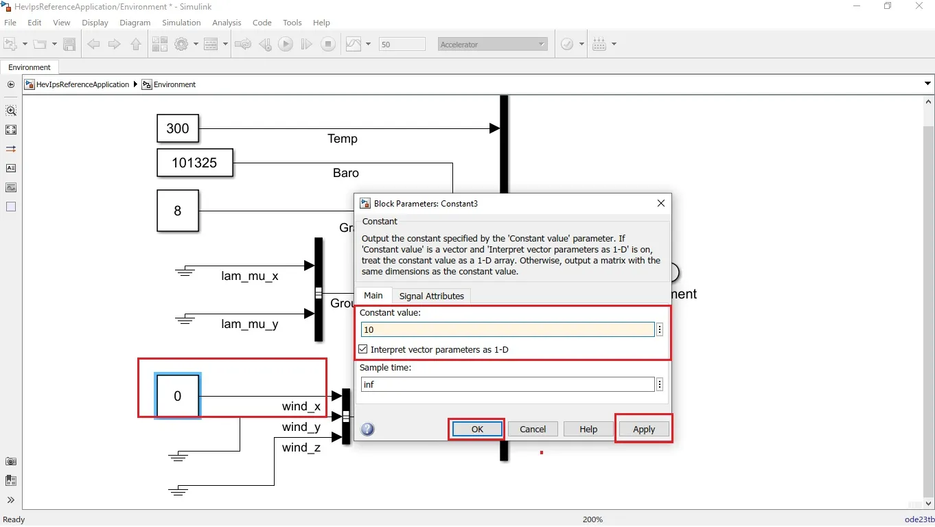
The wind velocity = 10 m/s.
Results:
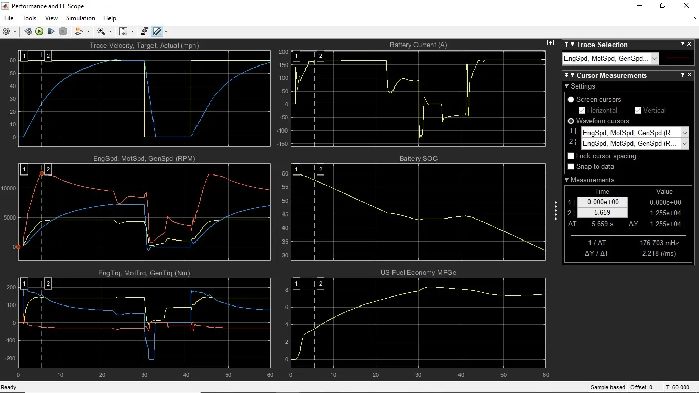
In all the results some changes can be observed as that of previous results. Though the drive cycle parameters are the same, some changes in the environment block such as grade angle and wind velocity lead to changes in final results.
Plot 1: Trace Velocity, Target, Actual(mph)
It shows the velocity of the vehicle for the Drive cycle data with the Time scale on the x-axis.
Traced velocity is given as input command & actual velocity is output. The actual graph doesn’t match with input traced velocity due to limited instantaneous current/power available.
The top speed achieved = 60 mph
The acceleration time to reach 60 mph = 22.21 seconds
The deceleration time from 60 to minimum = 2.79 seconds
It can be observed that the top speed achieved with these conditions is less than the earlier case and time required to reach the top speed is also higher. The vehicle does not reach the desired velocity which can be attributed to the steep gradeability and high resistance force by the wind.
Plot 2: Engine Speed, Motor Speed, Generator Speed(RPM)
It shows the changes in the speed of the engine, motor and generator in rpm throughout the drive cycle.
Peak Engine speed = 4651 Rpm
Peak Motor speed = 7295 Rpm
Peak Generator speed = 12550 Rpm
The motor initiates the initial acceleration to produce propulsion power to reach the specified maximum velocity, but it can be observed that the motor is unable to produce enough propulsion power to reach the desired velocity, thus the engine contributes to the propulsion effort. However, the combined effort is not sufficient to reach the desired velocity due to resistance offered by wind velocity and grade angle.
Plot 3: Engine Torque, Motor Torque, Generator Torque(Nm)
It shows the torque characteristics and its changes of engine, motor and generator in (Nm) throughout the drive cycle.
Peak Engine torque = 145 Nm
Peak Motor torque = 202 Nm
Peak Generator torque = 52.67 Nm
With Wide-open throttle specification, the motor runs at maximum torque, however, the power distribution stabilizes between the motor and the engine as the vehicle reaches the desired velocity as earlier mutual stabilization point is not observed as the specifications of the drive cycle are not met. A negative value for the generator indicates the engine torque is used to charge the battery as well during the propulsion time.
Plot 4: Battery Current (A)
It shows the battery current values (A) and its changes for various acceleration inputs as per the Drive cycle.
The peak current discharge from the battery = 166 A
The peak current charging to the battery = -125.37 A
With Wide-open throttle specification, the powertrain draws maximum current from the battery, here maximum energy discharge period lasts longer indicating that the motor specifications and control strategy are not sufficient to meet the specifications. A negative battery current value indicates regenerative braking and charging by the engine.
Plot 5: Battery SOC
It shows the battery state of charge SOC (%) and its changes corresponding to the driving inputs.
The state of charge decreased from 60% to 28% of charge in 60 seconds, for the specified driving conditions.
Plot 6: US Fuel economy MPGe
Shows the Fuel Economy as Mile per Gallons for the corresponding input driving conditions.
According to the drive cycle, the vehicle achieved its maximum speed after 22 seconds and the speed is constant up to 30 seconds of drive cycle (from plot 1), so it can be observed(from plot6) that fuel requirement is also increasing with the increase in speed till the speed is constant. After this constant speed vehicle speed is decreasing and the vehicle is at lowest speed for next 10-12 seconds and during this, the fuel requirement is also decreasing, and the same drive cycle and fuel requirement is repeated.
Conclusion:
According to the simulation results for both the cases i.e with and without grade angle & wind velocity, it can be said that vehicle in which grade angle and wind velocity is equal to zero is more efficient than the former one.
- In case II, due to wind velocity and Gradeability, the vehicle is not able to match the targeted speed.
- In case II, maximum rpm achieved by the motor is less because of resistance offered by grade angle & wind velocity, while an engine & generator is a bit less than the case I but we can consider it as same due to negligible difference.
- In case II, the battery current is almost the same. As battery have the same max capacity in both the cases.
- In Case II the state of charge also shows that the discharge is also high compared to the case I.
- MPGe achieved is less in case II than the case I in the same period it is because of the resistance offered by grade angle & wind velocity.
- So overall we can say that adding gradeability & wind resistance causes the vehicle to achieve less acceleration & top speed at same battery capacity & MPGe achieved is also less(vehicle becomes less economic).
- It can be observed that the efficiency of the no-load vehicle is high compared to the vehicle with additional loads acting on them.
Q4. Keeping all other parameters same, compare the simulated results of hybrid and pure electric powertrains.
Pure Electric Vehicle:
An electric vehicle (EV) is a vehicle that uses one or more electric motors or traction motors for propulsion. An electric vehicle may be powered through a collector system by electricity from off-vehicle sources, or maybe self-contained with a battery, solar panels, fuel cells or an electric generator to convert fuel to electricity. EVs include, but are not limited to, road and rail vehicles, surface and underwater vessels, electric aircraft and electric spacecraft.
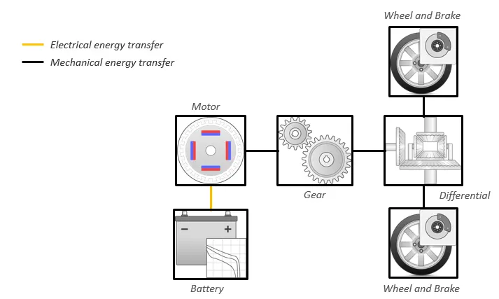
In MATLAB using Powertrain Blockset - Design tradeoff analysis and component sizing, control parameter optimization, or hardware-in-the-loop (HIL) testing for the fully electric vehicle under that exploring Electric Vehicle Input Power-Split Reference Application.
Selecting - autoblkevStart
Simulation Model:
Simulation Condition:
Since comparing an electric vehicle against a hybrid electric vehicle, it is important to have a level playing field. Thus, running the vehicle along the same drive cycle and comparing variables that are important to the consumer and the environment i.e. efficiency, range and MPGe.
For the first block keeping the input drive cycle i.e Wide Open Throttle(WOT) same as used earlier, Changing the grade and wind velocity, keeping all other parameters as default.
The simulation is done for Hybrid electric vehicle with Wide open Throttle Drive cycle.
The Total cycle time = 60 seconds
Time to start deceleration = 30seconds
The Grade angle = 8 Degrees
The wind velocity = 10 m/s.
Results:
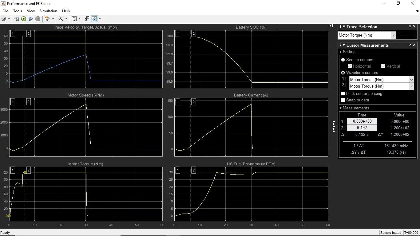
Plot 1: Trace Velocity, Target, Actual(mph)
It shows the velocity of the vehicle for the Drive cycle data with the Time scale on the x-axis.
Traced velocity is given as input command & actual velocity is output. The actual graph doesn’t match with input traced velocity due to limited instantaneous current available.
The top speed achieved = 35 mph
The acceleration time to reach 35 mph = 30 seconds
The deceleration time from 35 to minimum = 2.28 seconds
Plot 2: Motor Speed(RPM)
It shows the changes in the speed of the engine, motor and generator in rpm throughout the drive cycle.
Peak Motor speed = 3415 Rpm
Plot 3: Motor Torque(Nm)
It shows the torque characteristics and its changes of engine, motor and generator in (Nm) throughout the drive cycle.
Peak Motor torque = 120 Nm
A negative torque is seen after 30 seconds it is due to regenerative braking.
Plot 4: Battery SOC
It shows the battery state of charge SOC (%) and its changes corresponding to the driving inputs.
The state of charge decreased from 100% to 99% of charge in 60 seconds, for the specified driving conditions.
Plot 5: Battery Current (A)
It shows the battery current values (A) and its changes for various acceleration inputs as per the Drive cycle.
The peak current discharge from the battery = 139 A
It can be seen that after 30 sec the battery current has gone in negative it is due to regenerative braking.
Plot 6: US Fuel economy MPGe
Shows the Fuel Economy as Mile per Gallons for the corresponding input driving conditions.
Here there is no fuel in the pure electric vehicle however this gives equivalent battery energy required that of the fuel energy, and calculates the Fuel efficiency.
According to the drive cycle, the vehicle achieved its maximum speed after 30 seconds and suddenly the speed is decreasing next 2 and half seconds (from plot 1), so it can be observed(from plot6) that fuel requirement i.e power from the battery in this pure electric vehicle is also increasing with the increase in speed till speed reaches at peak and during the sudden decrease in speed the power requirement value is also getting decreased.
Comparison and conclusion for Pure electric vs Hybrid vehicle with same conditions:
1. In a full-electric vehicle, less top speed is achieved as compared to HEV. The electric vehicle is capable of producing more values of Motor speed and Motor torque compared to the hybrid vehicle's motor alone, but hybrid electric vehicle combines the torque of both motor and it's the engine it is higher than the electric vehicle's torque, this helps in pulling the HEV at higher top speed as compared to the pure electric.
2. As the pure electric car uses Lithium-ion battery and HEV uses the Nickel-metal hydride battery, the discharging capacity and the rate of charging is higher in the pure electric car. As it can discharge at a fast rate the motor can produce a high amount of torque instantly compared to the HEV. Battery SOC plot shows the battery efficiency of the pure electric to be higher than the HEV and this is also due to the battery type used in these cars.
3. The efficiency of the electric car is higher than the HEV which is evident from the miles per gallon numbers of both of these cars.
4. The electric vehicle produces zero emissions whereas the hybrid one's produce waste gas emission.
Conclusion-
- Mapped model is simple & suitable for the static problem where we can compromise on accuracy while dynamic is suitable for complex problems requires high accuracy.
- Miles per gallon block uses data from vehicle speed & battery power in MPGe.
- Adding gradeability & wind resistance causes the vehicle to achieve less acceleration & top speed at same battery capacity & MPGe achieved is also less(vehicle becomes less economic).
- The electric vehicle is best suited where initial acceleration & max power is not much of importance & MPGe is required at higher side. While on another hand, Hybrid vehicle is best suited where initial acceleration & max power is an important factor with little compromising on MPGe. So pure electric vehicle is more economical.