Genetic Algorithm
Aim:-To optimise the stalagmit function and find the global maxima using 'Genetic Algorithm'.
And explain the concept of genetic algorithm and also explain the syntax for ga in MATLAB.
Genetic Algorithm:-
In a genetic algorithm, a population of candidate solutions (called individuals, creatures, organisms, or phenotypes) to an optimization problem is evolved toward better solutions. Each candidate solution has a set of properties (its chromosomes or genotype) which can be mutated and altered; traditionally, solutions are represented in binary as strings of 0s and 1s, but other encodings are also possible.
The evolution usually starts from a population of randomly generated individuals, and is an iterative process, with the population in each iteration called a generation. In each generation, the fitness of every individual in the population is evaluated; the fitness is usually the value of the objective function in the optimization problem being solved. The more fit individuals are stochastically selected from the current population, and each individual's genome is modified (recombined and possibly randomly mutated) to form a new generation. The new generation of candidate solutions is then used in the next iteration of the algorithm. Commonly, the algorithm terminates when either a maximum number of generations has been produced, or a satisfactory fitness level has been reached for the population.
A typical genetic algorithm requires:
a genetic representation of the solution domain,
a fitness function to evaluate the solution domain.
A standard representation of each candidate solution is as an array of bits (also called bit set or bit string).[3] Arrays of other types and structures can be used in essentially the same way. The main property that makes these genetic representations convenient is that their parts are easily aligned due to their fixed size, which facilitates simple crossover operations. Variable length representations may also be used, but crossover implementation is more complex in this case. Tree-like representations are explored in genetic programming and graph-form representations are explored in evolutionary programming; a mix of both linear chromosomes and trees is explored in gene expression programming.
Once the genetic representation and the fitness function are defined, a GA proceeds to initialize a population of solutions and then to improve it through repetitive application of the mutation, crossover, inversion and selection operators.
Syntax of genetic algorithm
[x fval] = ga(@fitnessfun, nvars, options)
where
• @fitnessfun is a handle to the fitness function.
• nvars is the number of independent variables for the fitness function.
• options is a structure containing options for the genetic algorithm. If you do not
pass in this argument, ‘ga’ uses its default options.
The results are given by
• x — Point at which the final value is attained
• fval — Final value of the fitness function
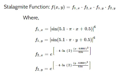
Stalagmit Function:-
function[f]=stalagmit(input_vector)
x=input_vector(1);
y=input_vector(2);

f1_x=(sin(5.1*pi*x+0.5))^6;
f1_y=(sin(5.1*pi*y+0.5))^6;

f2_x=exp(-4*log(2)*((x-0.0667)^2)/0.64);
f2_y=exp(-4*log(2)*((y-0.0667)^2)/0.64);

f=-(f1_x*f1_y*f2_x*f2_y);
end
Main Program:-
close all
clc
%Difining our search space

x=linspace(0,0.6,150);
y=linspace(0,0.6,150);

%creating a 2D mesh
[xx,yy]=meshgrid(x,y);

%evaluating stalaggmit function
for i=1:length(xx)
    for j=1:length(yy)
        input_vector(1)=xx(i,j);
        input_vector(2)=yy(i,j);
        f(i,j)=stalagmit(input_vector);
    end
end

%case1-unbounded inputs
% number of iterations
num_cases_1=50;
tic
for i=1:num_cases_1
    [inputs,fopt_1(i)]=ga(@stalagmit,2);
    xopt(i)=inputs(1);
    yopt(i)=inputs(2);
end
fopt_1=-fopt_1;
study_time=toc

figure(1)
subplot(2,1,1)
hold on
surfc(x,y,-f)
shading interp
plot3(xopt,yopt,fopt_1,'marker','o','MarkerSize',5,'MarkerFaceColor','r')
title('unbounded inputs')
subplot(2,1,2)
plot(fopt_1)
xlabel('ITERATIONS')
ylabel('FUNCTION MAXIMUM')

%study 2 Bounded inputs

tic
for i=1:num_cases_1
    [inputs2,fopt_2(i)]=ga(@stalagmit,2,[],[],[],[],[0,0],[1,1]);
    xopt2(i)=inputs2(1);
    yopt2(i)=inputs2(2);
end
fopt_2=-fopt_2;
study_time2=toc

figure(2)
subplot(2,1,1)
hold on
surfc(x,y,-f)
shading interp
plot3(xopt2,yopt2,fopt_2,'Marker','o','MarkerSize',5,'MarkerFaceColor','r')
title('Bounded inputs')
subplot(2,1,2)
plot(fopt_2)
xlabel('Iteration')
ylabel('FUNCTION MAXIMUM')

%study 3 maximising the population size to otimise result
options=optimoptions('ga');
options=optimoptions(options,'PopulationSize',350);
tic
for i=1:num_cases_1
    [inputs3,fopt_3(i)]=ga(@stalagmit,2,[],[],[],[],[0,0],[1,1],[],[],options);
    xopt3(i)=inputs3(1);
    yopt3(i)=inputs3(2);
end
fopt_3=-fopt_3;

figure(3)
subplot(2,1,1)
hold on
surfc(x,y,-f)
shading interp
plot3(xopt3,yopt3,fopt_3,'Marker','o','MarkerSize',5,'MarkerFaceColor','r')
title('MAXIMISING POPULATION')
subplot(2,1,2)
plot(fopt_3)
xlabel('Iteration')
ylabel('FUNCTION MAXIMUM')Refrences:-https://https://www.bing.com/search?