Week 3 - Taylor table method and Matlab code

Intro: the numerical solution will give only answers at describing points in the domain which are called grid points. The finite difference method is for replacing the partial derivatives appearing in governing equations of fluid dynamics, with algebraic difference quotients yielding a system of algebraic equations that can be solved for the flow field variables at the specific, discrete grid points in the flow.

SCHEMES FOR FOUTH ORDER APPROXIMATION FOR SECOND ORDER DERIVATIVE:

We are having a set of grid points in our numerical stencil along the x-axis. Each grid points has its own Taylor series func. We first create a Taylor table from these sets of grid points as mentioned below

1. Central difference scheme:

	F(i)	F’(i)*d(x)	F’’(i)*d(x)^2	F’’’(i)*d(x)^3	F’’’’(i)*d(x)^4
F(i-2)	a	-2a	4a/2	-8a/2	16a/24
F(i-1)	B	-b	b/2	-b/6	b/24
F(i)	C	0	0	0	0
F(i+1)	D	D	d/2	d/6	d/24
F(i+2)	E	2e	4e/2	8e/6	16e/24
	0	0	1	0	0

The output of the code we get If we calculate it as a matrix The output will be

-1/12

4/3

-5/2

4/3

-1/12

2. skewed right difference scheme:

	F(i)	F’(i)*d(x)	F’’(i)*d(x)^2	F’’’(i)*d(x)^3	F’’’’(i)*d(x)^4	F’’’’’(i)*d(x)^5
F(i)	a	0	0	0	0	0
F(i+1)	B	B	b/2	b/6	b/24	b/120
F(i+2)	C	2c	4c/2	8c/6	16c/24	32c/120
F(i+3)	D	3d	9d/2	27d/6	81d/24	243d/120
F(i+4)	E	4e	16e/2	64e/6	25e/24	1024e/120
F(i+5)	G	5g	25g/2	125g/6	625g/24	3125g/120

The output will be for the code If we calculate it as a matrix The output will be

15/4

-77/6

107/6

-13

61/12

-5/6

3. Skewed left difference scheme:

	F(i)	F’(i)*d(x)	F’’(i)*d(x)^2	F’’’(i)*d(x)^3	F’’’’(i)*d(x)^4	F’’’’’(i)*d(x)^5
F(i)	a	0	0	0	0	0
F(i+1)	B	-B	b/2	-b/6	b/24	-b/120
F(i+2)	C	-2c	4c/2	-8c/6	16c/24	-32c/120
F(i+3)	D	-3d	9d/2	-27d/6	81d/24	-243d/120
F(i+4)	E	-4e	16e/2	-64e/6	-25e/24	-1024e/120
F(i+5)	G	-5g	25g/2	-125g/6	625g/24	-3125g/120
	0	0	1	0	0	0

If we calculate it as a matrix the output will be

15/4

-77/6

107/6

-13

61/12

-5/6

The partial derivative are written for scheme which are of 2^nd ode and 4^th ode approx... For approximating a derivative to an arbitrary order of accuracy we use finite difference. For the given problem we say that it is of 4^th ode accuracy because terms of the order 5 or more are completely neglected here. Each column in a table has 5 unknowns. An algebraic equation is formed with these unknowns. If equations are formed for each and every column in a table we end up with a system of equations which is called a matrix. With help of a matrix, the values of unknowns are calculated.

Objective:

1. We are going to write a code to get the second-ode derivative of the analytical function exp(x)*cos(x) and compare it within 3 numerical approximations that what we derived.

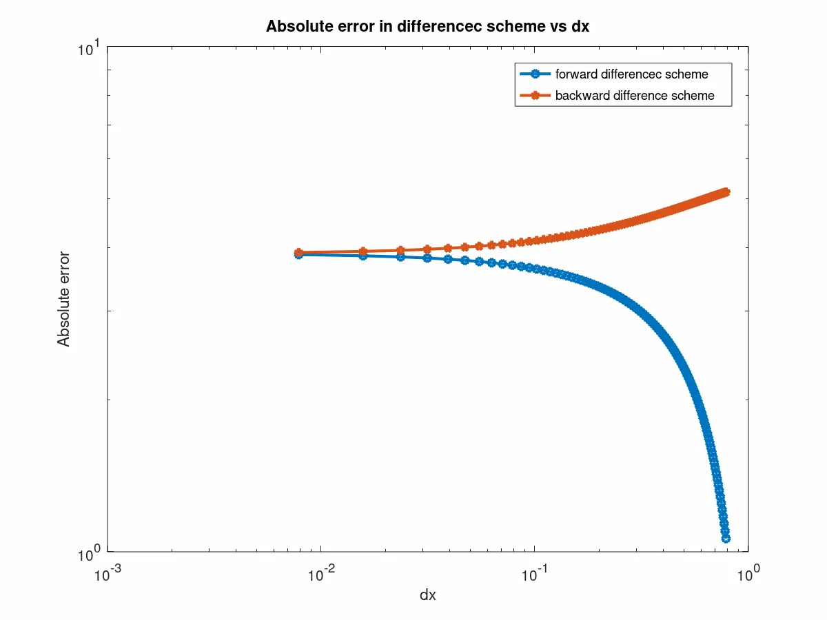
2, In the first plot for schemes that take only one grid points in the forward or backward direction in a numerical stencil along the x-axis we can tell that ass the value of dx keep on increasing the absolute value of the error will vary at a rapid rate by either increasing or ode until that value of dx reaches and then that the value of absolute error becomes unstable for different schemes.

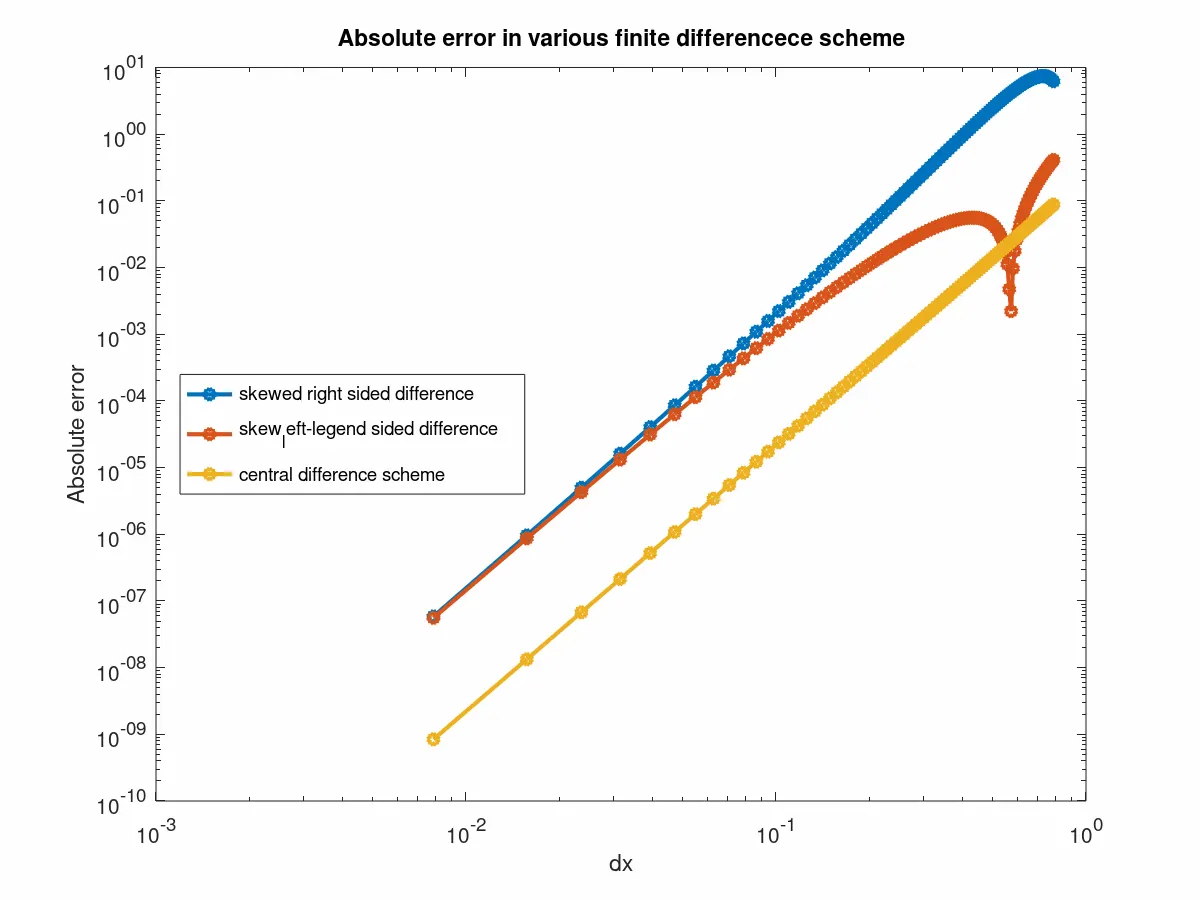
3. In the second plot, the value of absolute error is less for the central difference and it increases for the skewed schemes. For a range of dx values, the plots are linear in central (CDS) and start 10^-9 but for the skewed schemes, the values of abs error will be unstable.
4. The linear plot will not be the same if the value of dx becomes greater than 1 and because of which the absolute error values will become unstable.
5. The improvement of approximation quality is due to the node(i) being at a closer distance which is observed in the case of central(CDS) separated by a distance of 2 grid points apart, but for the skewed schemes since the distance to the node(i) is 5 grid points apart which is the reason behind the absolute value for errors higher.
6. The slope of the curve will remain constant at 4 when the log values of dx keep on increasing for the various finite difference schemes.

Uses of skewed schemes:

When data from the rid points is only available from either the left or right end i.e. at nodes closer to the boundaries for computations that require a high order approximation we make use of skewed schemes.

Having asymmetric stencil for computation is not possible in this we do central (CDS) will give a lower order accuracy. For consistency of scheme to be maintained the values of dx are kept as low as possible for providing proper commutations.

I Conclude that a fourth-order approximation is derived for 2^nd ode making use of the Taylor table method will give a higher accuracy for simple computations, but for complex calculation, we need to go with lower ode approximation.