Week 9 - FVM Literature Review

Aim: To describe the need for interpolation schemes and flux limiters in the finite volume method.

Difference between finite difference method and finite volume method:

 FDM is a differential scheme, that is an approximation of a Taylor series expansion. You try to write the first order, second order differential in terms of the difference between two point values. This may bring in some approximation error.

The Finite Volume method is an integral scheme. Since you are integrating across the area, the chance of error is minimized.

Theory:

Discretization is the process of converting partial differential equations into an algebraic form the whole idea behind the discretization is to get the solution at the discrete point.

There are three types of discretization methods those are

1. Finite difference method: simple, straightforward to apply, and structured grids.

2. Finite element method: Applied to any geometries.

3. Finite volume methods: conservative and applied to any geometries.

Finite volume method:

In the case of FVM, the problem domain is divided into a number of non-overlapping control volumes called finite volume. Finite volume is based upon the approximate solution of the integral form of the conservation equation. the integral form of conservation law for control volume involves both surface and volume integral.

The differential equation is integrated over each control volume. Otherwise, profiles expressing the variation of the unknown between the grid points are used to evaluate the required integrals. Integral occurring in the conservation equations are evaluated using function values at computational nodes.

Finite volume refers to small volume surroundings each node points on a mesh. In Fvm equations are written in entire volume and no assumption was made over the shape of the volume. Inside this particular volume, all the flow and flow quantities are conserved.

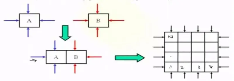
Consider 2 particular finite volumes A and B as shown in the figure. The flux is going in and out of the volume to get a complete set of domains or grids all the individual volumes like A and B are combined.

Features of FVM:

1. FVM can accommodate any type of grid and hence it is naturally suitable for any type of grid.
2. Unstructured grid generation methods and mesh partitioning techniques developed for the finite element method can be directly used in FVM.

Interpolation method:

The approximation of surface and volume integrals require values of the variable ate locations other than The computational nodes of the control volume.

Values at these locations are obtained using the interpolation formula.

Various possibilities for interpolation e.g.

1. Upwind interpolation
2. linear interpolation
3. Quadratic upwind interpolation
4. Hybrid, TVD, and ENO interpolation schemes.

Upwind interpolation:

UDS is equivalent to using a backward or forward finite difference approximation (depending on the flow of direction)

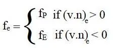
The advantage of upwind interpolation is the only approximation satisfies the boundness criterion unconditionally.

Disadvantages are

1. numerically diffusive and numerical diffusion is magnified in multidimensional problems if the flow is oblique to the grid.
2. Peak or rapid variations in the variables will be smeared out.
3. Only first-order is accurate. Hence very fine grids are required to obtain accurate solutions.
4. Approximate the values of the variable at cv face enter by linear interpolation of the values at two nearest computational nodes.
5. The linear interpolation is equitant to the use of the central difference formula of the first-order derivative and hence, this scheme is also a difference scheme(CDS).

Linear interpolation:

This scheme uses central difference formula and hence it is also termed a central difference scheme (CDS). It is one of the schemes used to solve the integrated convection-diffusion equation. The advantages of this method are that it is easy to understand and to implement at least for simple material relations. And its convergence rate is faster than some other finite differencing methods, Tylor series truncation error of the central differencing scheme is the second order

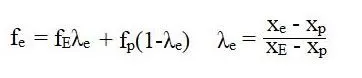
Characteristics of linear interpolation

1. CDS is second-order accurate
2. It may produce oscillatory solutions.
3. Simplest and most widely used interpolation
4. This leads to a very simple approximation for the evaluation of the gradient required for the evaluation of diffusive fluxes.
5. The approximation of gradients has second-order accuracy on uniform grids.
6. It's formally first order on non-uniform grids.

Quadratic upwind interpolation:

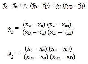
In this case, we have to approximate the value of the variable at the control volume face center by quadratic interpolation of the values at three nearest computational nodes (one downstream node D and 2 upstream nodes U and UU)

 

Hybrid scheme:

This scheme is a combination of a central difference scheme and an upwind difference scheme. It makes use of CDS, which is second-order accurate for small peclet numbers (Pe<2). For large peclet numbers(Pe<2) it uses the upwind difference scheme, which is first-order accurate but takes into account the convection of the fluid.

 

Total variation Diminish(TVD):

TVD scheme is employed to capture sharper shock predictions without any misleading oscillations when the variation of field variables is discontinuous. To capture the variation fine grids (delta x =very small) are needed and the computation becomes heavy and therefore uneconomic. The use of coarse grids with CDS, upwind scheme, hybrid difference scheme gives false shock predictions. (TVD) scheme enables sharper shock predictions on coarse grids saving computations time and as the scheme preserves monotonicity there are no spurious oscillations in the solution.

Flux limiter:

These are used in high-resolution schemes. i.e. numerical schemes used to solve the problem in science and engineering particularly fluid dynamics, described by PDE. They are used in high-resolution schemes, such as the MUSCL scheme, to avoid the spurious oscillations(wiggles) that would, otherwise occur with high-order spatial discretization schemes due to shocks, discontinuities, or sharp changes in the solution domain. The use of flux limiters, together with an appropriate high-resolution scheme, makes the solution total variation diminishing (TVD).

 

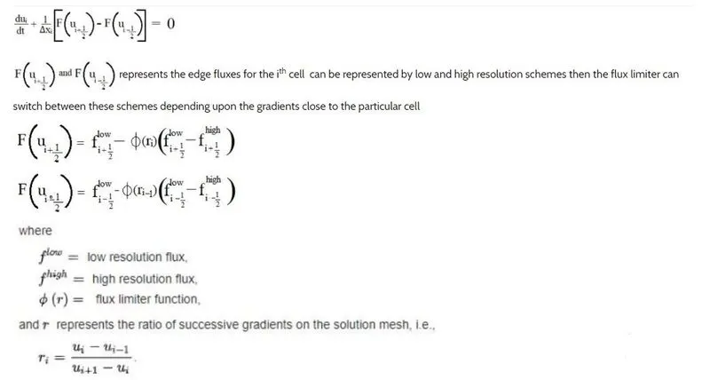
Note that flux limiters are also referred as slope limiters because they both have the same mathematical form, and both have the effect of limiting the solution gradient near shock or discontinuities, in general, the term flux limiter is used when the limiter acts on system states (like pressure, velocity, etc)

Need of interpolation schemes and flux limiters in FVM:

1. The gauss or divergence theorem simply states that the outward flux of a vector field through a closed surface is equal to the volume integral of the divergence over the region inside the surface.
2. This theorem is fundamental in the FVM, it is used to convert the volume integrals appearing in the governing equation into surface integrals.
3. The face value appearing in the convective and diffusive fluxes has to be computed by some form of interpolation from the centroid values of the control volume at both sides of the faces.
4. After special discretization, we can proceed with temporal discretization. By proceeding in this way we are using the method of lines(MOL)
5. The main advantage of the MOL method is that it allows us to select numerical approximations of different accuracy for the spatial and temporal terms. Each term can be treated differently to yield different accuracies.
6. Nearly all flows in nature and industrial applications are unsteady ( also known as transient or time-dependent)

Unsteadiness due to:

Instabilities

Non-equilibrium initial conditions, time–dependent boundary conditions, source term, chemical reactions, moving or deforming bodies, turbulence, buoyancy, convection, multiple phases.