Project 2 - Rankine cycle Simulator

Rankine cycle - the Ideal Cycle for Vapor Power Cycle

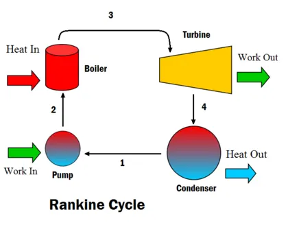
Vapor power plants generate electrical power by using fuels like coal, oil or natural gas. The schematic of a vapor power plant is shown on the left. The entire power plant can be broken down into four major subsystems.

• Subsystem A: Energy conversion from heat to work
• Subsystem B: Energy source and waste removal required to vaporize the water
• Subsystem C: Electric generator
• Subsystem D: Cooling water system

The focus of this chapter is subsystem A. The thermodynamic cycle in subsystem A is called the Rankine cycle. Subsystem A consists of a boiler, turbine, condenser, and pump. Fuel, burned in the boiler, heats the water to generate superheated steam (subsystem B). This steam is used to run the turbine which powers the generator. Electrical energy is generated when the generator windings rotate in a strong magnetic field (subsystem C). After the steam leaves the turbine, it is cooled to its liquid state in the condenser by transferring heat to the cooling water system (subsystem D). The liquid is pressurized by the pump prior to going back to the boiler.

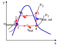
• 1-2: Isentropic compression in a pump
• 2-3: Constant pressure heat addition in a boiler
• 3-4: Isentropic expansion in a turbine
• 4-1: Constant pressure heat rejection in a condenser

Pump (process 1-2): Pump pressurized the liquid water from the condenser prior to going back to the boiler. Assuming no heat transfer with the surroundings, the energy balance in the pump is

w_{pump, in} = h₂ - h₁

Boiler (process 2-3): Liquid water enters the boiler and is heated to superheated state in the boiler. The energy balance in the boiler is

q_in = h₃ - h₂

Turbine (process 3-4): Steam from the boiler, which has an elevated temperature and pressure, expands through the turbine to produce work and then is discharged to the condenser with relatively low pressure. Neglecting heat transfer with the surroundings, the energy balance in the turbine is

w_{turbine, out} = h₃ - h₄

Condenser (process 4-1): Steam from the turbine is condensed to liquid water in the condenser. The energy balance in the condenser is

q_out = h₄ - h₁

For the whole cycle, the energy balance can be obtained by summarizing the four energy equations above. It yields,

(q_in- q_out) - (w_{turbine, out} - w_{pump, in}) = 0

The thermal efficiency of the Rankine cycle is determined from

η_th = w_{net ,out}/q_in = 1 - q_out/q_in

Where the network output from the cycle is

w_{net ,out} = w_{turbine, out} - w_{pump, in}

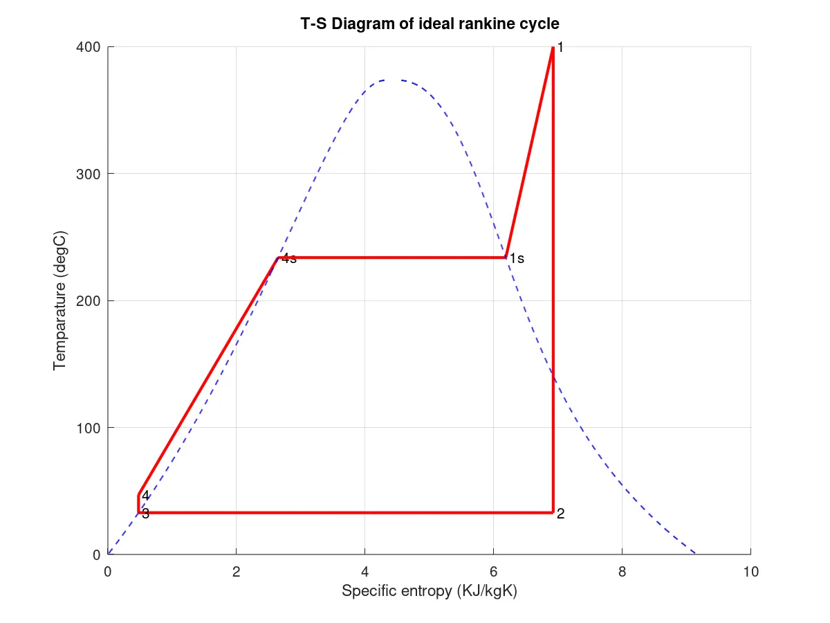
The Rankine cycle is an ideal cycle if water passes through the four components without irreversibilities and pressure drops. The ideal Rankine cycle consists of the following four processes, as shown on the T-s diagram on the left:

• 1-2: Isentropic compression in a pump
• 2-3: Constant pressure heat addition in a boiler
• 3-4: Isentropic expansion in a turbine
• 4-1: Constant pressure heat rejection in a condenser

clear all
close all
clc
%given inputs
P1=30;
P2=0.05;
T1=400;

%printing the all the state points as required
fprintf('\n       RANKINE CYCLE SIMULATOR');
fprintf('\n\n1-2 Isentropic Expansion in Turbine');
fprintf('\n2-3 Constant pressure heat rejection by the condensor');
fprintf('\n3-4 Isentropic compression in pump');
fprintf('\n4-1 constant heat addition at boiler\n');

%giving inputs
%taking all input arguments
P1=input('enter the pressure at the turbine inlet(in bar): ');
T1=input('enter the temparature at the turbine inlet (in degree): ');
P2=input('enter the pressure at the condenser(in bar): ');


fprintf('     RESULT\n');
%calculation for general properties
%step1
%calculation of Cp value at p1&p2 for saturated liquid and vapour

CP1_L=XSteam('CpL_p',P1);
CP1_V=XSteam('CpV_p',P1);
CP2_L=XSteam('CpL_p',P2);
CP2_V=XSteam('CpV_p',P2);




%calculation of enthalpy and entropy at saturation points
%step2
%calculation of saturation properties at state 1

Hg_1=XSteam('hV_p',P1);
Sg_1=XSteam('sV_p',P1);

%step3
%calculation of saturation properties at state 2

Hg_2=XSteam('hV_p',P2);
Sg_2=XSteam('sV_p',P2);

%step4

%calculation of saturation properties at state 3

Hf_3=XSteam('hL_p',P2);
Sf_3=XSteam('sL_p',P2);

%step5

%calculation of saturation properties at state 4
Hf_4=XSteam('hL_p',P1);
Sf_4=XSteam('sL_p',P1);

%calculation of process properties at state 1
%step6

fprintf('at state point 1\n');

fprintf('P1 is :%f bar\n',P1);
fprintf('T1 is :%f degC\n',T1);

H1=XSteam('h_pT',P1,T1);
fprintf('H1 is :%f KJ/kg\n',H1);

S1=XSteam('s_pT',P1,T1);
fprintf('S1 is :%f KJ/kgK\n',S1);

%calculation of process properties at state 2
%step7

fprintf('at state point 2\n');

fprintf('P2 is :%f bar\n',P2);

S2=S1;

fprintf('S2 is :%f KJ/kgK\n',S2);

Sf_2=XSteam('sL_p',P2);
Sg_2=XSteam('sV_p',P2);

Hf_2=XSteam('hL_p',P2);
Hg_2=XSteam('hV_p',P2);
x=(S2-Sf_2)/(Sg_2-Sf_2);
H2=Hf_2+(x*(Hg_2-Hf_2));
T2=XSteam('T_hs',H2,S2);
fprintf('T2 is : %f degC\n',T2);

%
fprintf('H2 is :%f KJ/kg\n', H2);

%calculation of process properties at state 3
%step 8

fprintf('at stste point 3\n');

P3=P2;
fprintf('p3 is :%f Bar\n', P3);
V3=XSteam('vL_p',P3);
H3=Hf_3;
S3=Sf_3;
T3=XSteam('T_hs',H3,S3);

fprintf('T3 is :%f degC\n', T3);

H3=Hf_3;
fprintf('H3 is :%f KJ/kg\n', H3);

S3=Sf_3;
fprintf('S3 is :%f KJ/kgK\n', S3);

%calculation of process properties at state 4
%step9
fprintf('at state point 4\n');

P4=P1;
fprintf('P4 is :%f Bar\n',P4);
S4=S3;
fprintf('S4 is :%f KJ/kgK\n', S4);

Wp=V3*(P4-P3)*100;
H4=Wp+H3;
fprintf('H4 is :%f KJ/kg\n', H4);
Tsat_P1=XSteam('Tsat_p',P1);
Tsat_P2=XSteam('Tsat_p',P2);

T4=(Tsat_P1+273.15)/(exp((Sf_4-S4)/CP1_L));
T4=T4-273.15;
fprintf('T4 is :%f degC\n', T4);

%calculating for plotting staturation liquid and vapour lines
%stp10

temp=linspace(1,T1,1000);

for i=1:length(temp)
  H_L(i)=XSteam('hL_T',temp(i));
  H_V(i)=XSteam('hL_T',temp(i));
  S_L(i)=XSteam('sL_T',temp(i));
  S_V(i)=XSteam('sV_T',temp(i));
end
%
%plotting T-S and H-S diagrams
%step11
%plotting T-S diagrams
figure(1)
hold on
plot([S1 S2],[T1 T2],'r','linewidth',2)
text(S1,T1,' 1')
text(S2,T2,' 2')

plot([S2 S3],[Tsat_P2 T3],'r','linewidth',2)
text(S3,T3,' 3')
plot([S3 S4],[T3 T4],'r','linewidth',2)
text(S4,T4,' 4')
plot([S4 Sf_4],[T4 Tsat_P1],'r','linewidth',2)
text(Sf_4,Tsat_P1,' 4s')
plot([Sf_4 Sg_1],[Tsat_P1 Tsat_P1],'r','linewidth',2)
text(Sg_1,Tsat_P1,' 1s')
plot([Sg_1 S1],[Tsat_P1 T1],'r','linewidth',2)
plot(S_L,temp,'b','linestyle','--','linewidth',1)
plot(S_V,temp,'b','linestyle','--','linewidth',1)

title('T-S Diagram of ideal rankine cycle')
ylabel('Temparature (degC)')
xlabel('Specific entropy (KJ/kgK)')
grid on
%srep12
%plotting H-S diagrams
figure(2)
hold on 
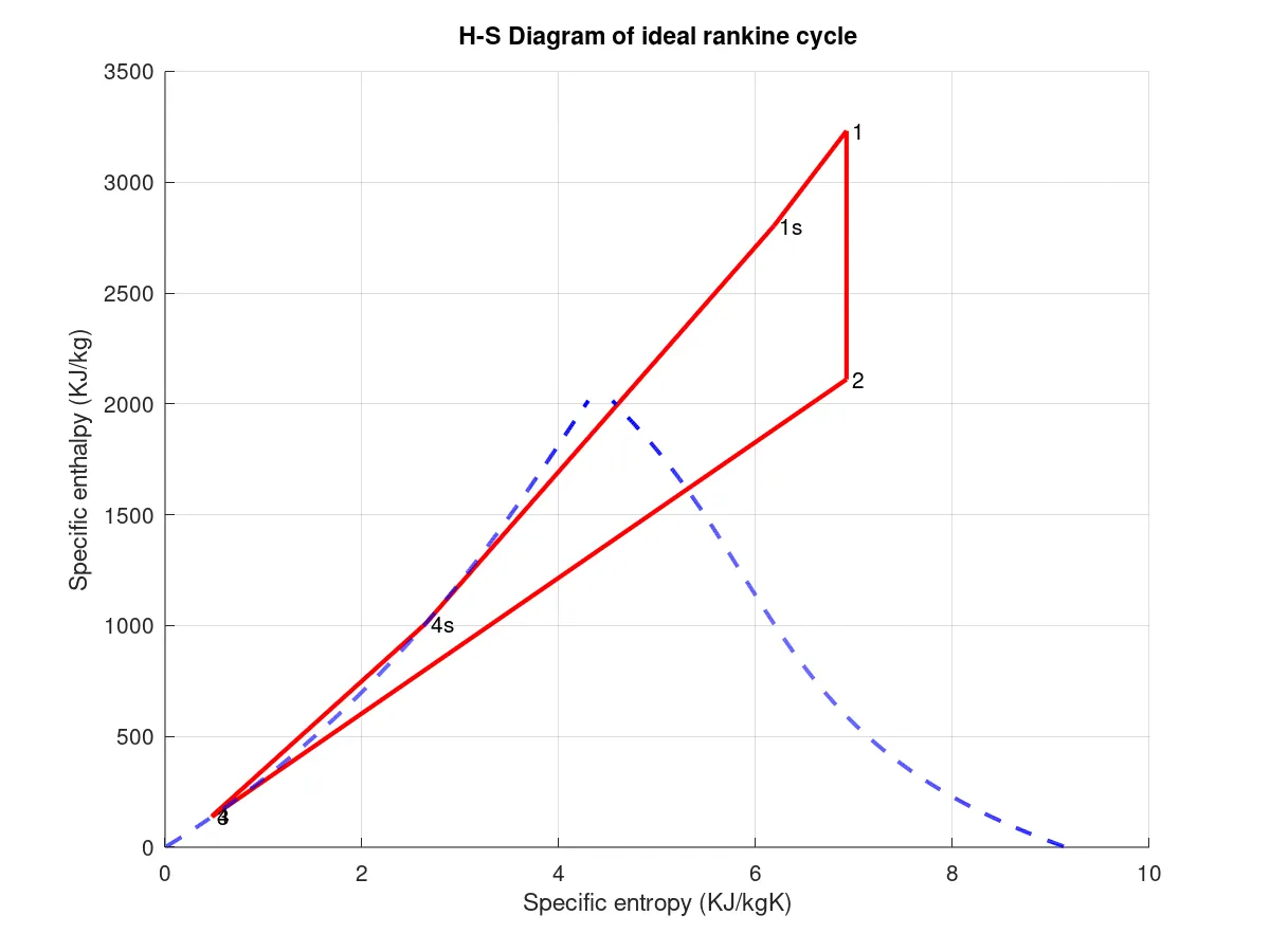
plot([S1 S2],[H1 H2],'r','linewidth',2)
text(S1,H1,' 1')
text(S2,H2,' 2')

plot([S2 S3],[H2 H3],'r','linewidth',2)
text(S3,H3,' 3')
plot([S3 S4],[H3 H4],'r','linewidth',2)
text(S4,H4,' 4')
plot([S4 Sf_4],[H4 Hf_4],'r','linewidth',2)
text(Sf_4,Hf_4,' 4s')
plot([Sf_4 Sg_1],[Hf_4 Hg_1],'r','linewidth',2)
text(Sg_1,Hg_1,' 1s')
plot([Sg_1 S1],[Hg_1 H1],'r','linewidth',2)
plot(S_L,H_L,'b','linestyle','--','linewidth',1.8)
plot(S_V,H_V,'b','linestyle','--','linewidth',1.8)
title('H-S Diagram of ideal rankine cycle')
ylabel('Specific enthalpy (KJ/kg)')
xlabel('Specific entropy (KJ/kgK)')
grid on
%work done,heat,SSC and efficiency calculation
%step13

Wt=H1-H2;
fprintf('work done by turbine is : %f KJ/kg\n',Wt)
fprintf('work done by pump is : %f KJ/kg\n',Wp)

Wnet=Wt-Wp
fprintf('net work done is :%f KJ/kg\n', Wnet)
Qin=H1-H4
eff_thermal=Wnet*100/Qin; %Efficiency
fprintf('Thermal efficiency is :%f', eff_thermal); disp('%')
SSC=3600/Wt; % specific stean consuption
fprintf('S.S.C is :%f kg/kwh\n', SSC)

Stepwise explanation:

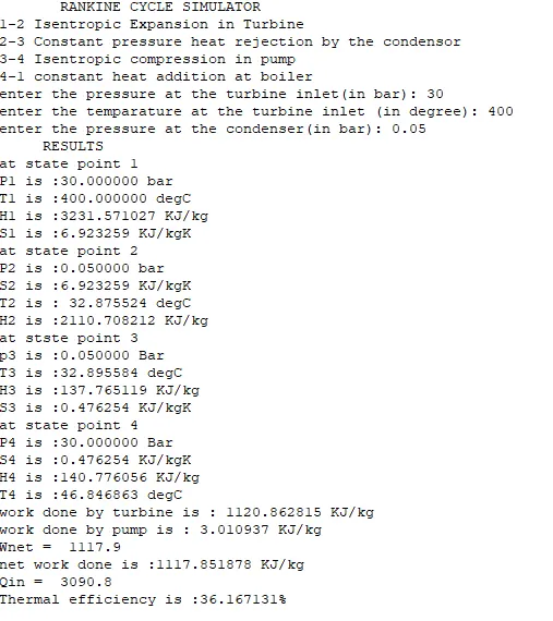
As a basic we are going to clear the workbook by using clear all command, then take input data as given p1 at turbine inlet is 30 bar and temperature t1 is 400 bar And condenser inlet p3 is 0.05 bar

Then by using fprintf command we are going to give the Rankine cycle title and their processes.

There are 4 processes in the cycle

1-2 Isentropic Expansion in Turbine

2-3 Constant pressure heat rejection by the condenser

3-4 isentropic compression in pump

4-1 constant heat addition at boiler

After that, by using the input command we are going to give all the given data values

Further from the XSteam data, we are going to extract the enthalpy, entropy, and temperature’s values

And as discussed in ideal Rankine theory at processes 1 to 2 entropy is constant so s1=s2

And work done is WT=h2=h1

From XSteam data file we can get the values of the variables in liquid and vapor values according to our processes requirements.

And at processes, 2 to 3 heat rejection processes q=h2-h3 and at processes 3 to 4 work done by the pump is Wp=h3-h4 entropy is constant, so by using all these equations we are going to calculate all the state point variables

Finally efficiency of the cycle Wnet/ qnet

And then by using plot commands we are going to plot the T-S and H-S diagram by using plot command and text commands used to give the state points, then title command gives the title of the plot. Then by using the labels command we are going to give the axis label.

Finally, our Rankine cycle plot is ready.

I conclude that the efficiency of a Rankine cycle will vary according to the liquid saturation temperatures. Why because these will affect the enthalpy and entropy values which result in turbine and pump performance.