Week 2 - Flow over a Cylinder.

Given Problem Statement:

1. Simulate flow over a cylinder for different Reynolds numbers by varying the velocity of the flow using a steady solver and calculate the drag and lift coefficient.
2. Simulate the flow over a cylinder for steady and unsteady solver and calculate the Strouhal Number for Re 100.
3. Study and discuss the effect of Reynold number on the coefficient of drag.
4. explain the effect of Von Karman Vortex Street.

Introduction to the project:

Flow over a cylinder body such as circular cylinder experiences boundary layer separation and flow oscillations in the wake region behind the body. When Reynolds number exceeds a threshold value flow motion developed in the wake region behind the body is a result of boundary layer separation from both sides of the body. This pattern of separation is called Von Karman Vortex Street. A Von Karman vortex street is repeating patterns of swirling vertices that are arising in the wake of flows around the blunt objects. The frequency of these oscillations is related to the Reynolds number of the flow which in this case depends on the velocity of the inlet flow.

Vortex Shedding:

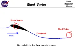
Vortex shedding is an oscillating flow that takes place when a fluid flows past a blunt body at a certain velocity. In this flow, the boundary layer separated from the surface forms a sheer layer that rolls into the vortex and detaches from the surface whereas in Von Karman Vortex Street shedding occurs from both the sides of the body which interact with each other. They shed alternatively from the cylinder and generates a regular vortex pattern called Karman Vortex Street.

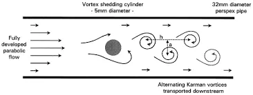
vortex street created by an aerodynamic object for reference;

visualization of the vortex street behind a circular cylinder in the air; the flow is made visible through the release of glycerol vapour in the air near the cylinder

Strauhal Number:

Strauhal number is the non-dimensional number describing the oscillating flow mechanism.

Sr=f⋅L/v

where Sr is Strauhal Number

f - frequency of oscillation in Hz

L - characteristic length in m.

In this case, L = D, where D is the diameter of the cylinder in m.

v - velocity in m/s

A large Strauhal number indicates that the viscosity dominates the flow whereas a lower Strauhal number indicates high-speed fluid.

Drag Coefficient.

Drag Coefficient is a dimensionless quantity that is used to quantify the resistance of an object. It is used in the drag equation which a lower drag coefficient indicates less aerodynamic or hydrodynamic drag.

The formula for Coefficient of drag (cd):

Cd=2.Fd/ρ.V2.A

where Fd is drag force in N.

ρ - density of the material in kg/m3kgm3

V - velocity of the inlet flow in m/s

A - area of the object in m2m2, here A is an area of a cylinder with a diameter of 2m.

Lift Coefficient.

The lift coefficient is a non-dimensionaless quantity that relates to the lifting force to the density of the fluid and velocity of the fluid and associated area of the object.

The formula for Coefficient of lift(Cl):-

Cl=2.Fl/ρ.V2.A

Where Fl is the lift force in N.

ρ- density of the material in Kg/m3

V - velocity of the inlet flow in m/s

A - area of the object in m2, here A is an area of a cylinder with a diameter of 2m.

Procedure:

Geometry:

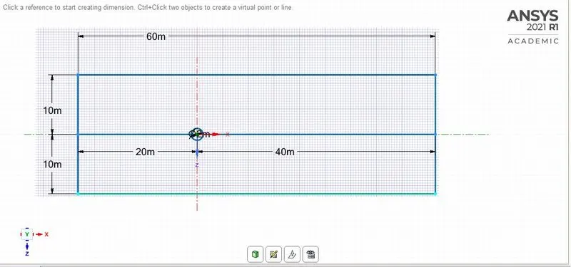
An infinitely long circular cylinder of diameter D=2.0 m is placed in an otherwise undisturbed uniform crossflow. The lateral boundary and the exit boundary in the far wake are placed at 10 D and 20D from the center of the circular cylinder, respectively. The cylinder is used to be drawn in SpaceClaim.

Dimensions of the Geometry:

Total length = 60m.

Total Width = 20m

Diameter of the cylinder = 2m.

Distance between inlet and center of the cylinder = 10D = 20m.

Distance between outlet and center of the cylinder = 20D = 40m.

Converting the geometry into the surface by using command pull and select. Also, delete the inside the circle to carry out the simulation.

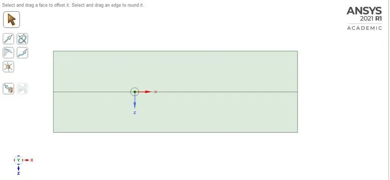
Then they select the construction line under the curves.

Mesh:

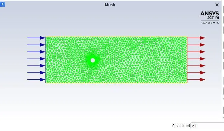
First of all, the baseline mesh autogenerated quad mesh was created. After that, it will change according to simulation requirements, and it was finely tuned with the help of triangular mesh generated. The model meshed with an element size of 0.25m.

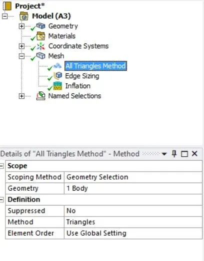
Edge sizing:

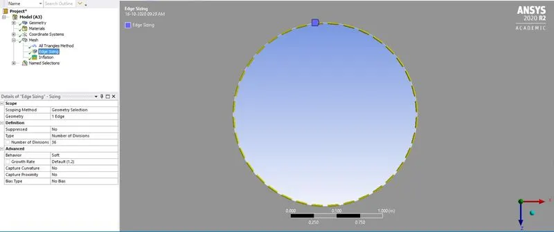
Body fitted mesh is generated by using the edge sizing command to make the cylinder wall smoother.

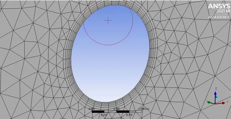
Inflation layer:

To capture the better results near the cylinder wall inflation layer set-up is used.

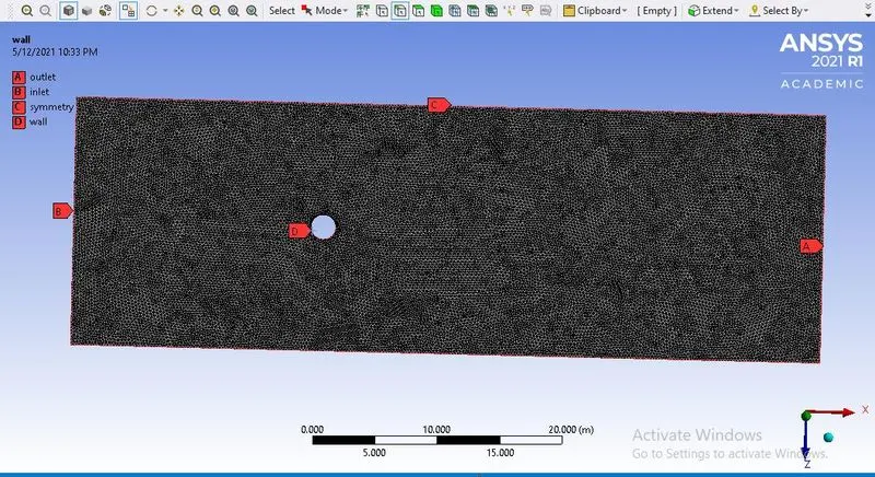
Named Selection of the created geometry and generating the finer mesh with a element size of 0.24m.

Setting up physics, boundary conditions and output:

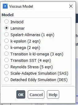
viscous model:

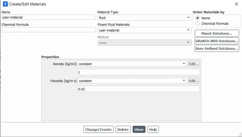
we are using a user-defined material type.

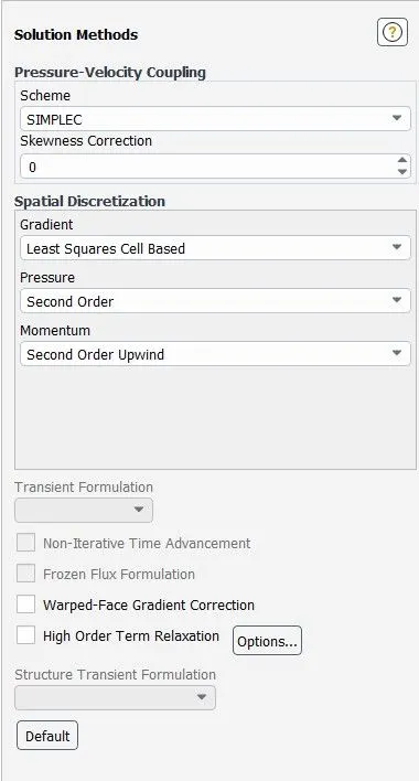
Solving method ( Unsteady state ):

For velocity-pressure coupling, the SIMPLEC algorithm was used. When the SIMPLEC algorithm is used, the pressure under-relaxation is automatically increased to 1.0. The setting for pressure under-relaxation is 0.3 (when the default SIMPLE algorithm is used). Here the momentum under-relaxation has also been increased from 0.7 to 0.9 to yield better convergence.

steady-state hybrid initialisation:

for the residual plot, we are going to uncheck the convergence values. to get the solution till the convergence.

Boundary condition type: Velocity inlet, pressure outlet.

The outlet pressure is set to gauge pressure of 0 Pascals. The sidewalls of the domain are assigned symmetry boundary conditions due to which velocity normal to the symmetry plane is zero and ensure zero gradient to all variables normal to the symmetry plane. The cylinder surface is assigned wall boundary conditions which is no-slip wall boundary condition.

Plots obtained using a steady solver.

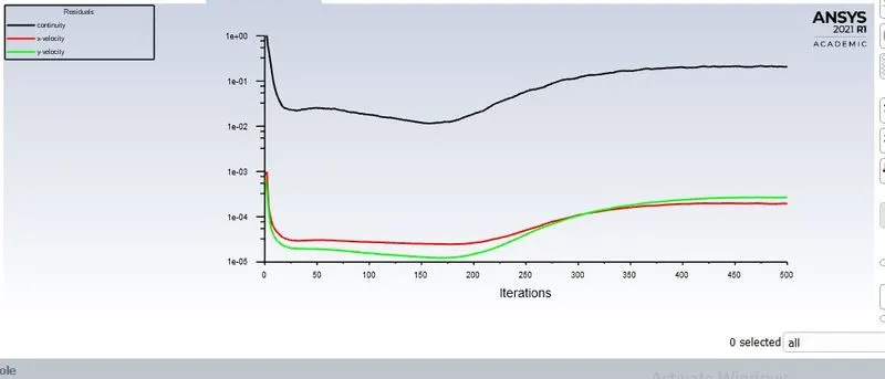
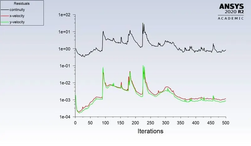
Residual Plot

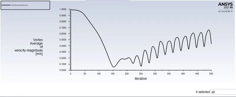
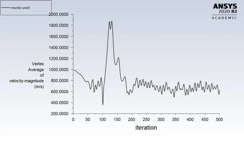
Velocity plot at the monitor point:

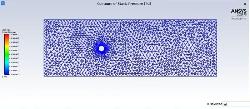
pressure contour:

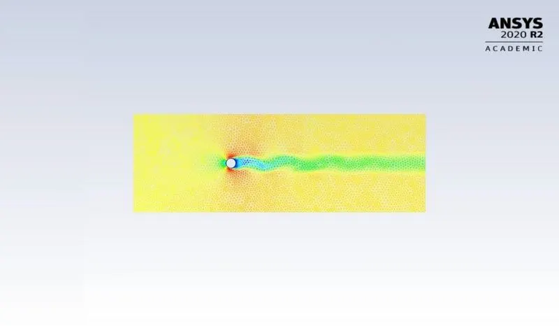
velocity contour plot:

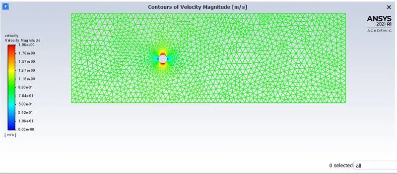
both plots are obtained from the initial condition

velocity contour at the final condition or after calculation

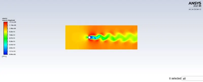
and then plots obtained by using the transient form:

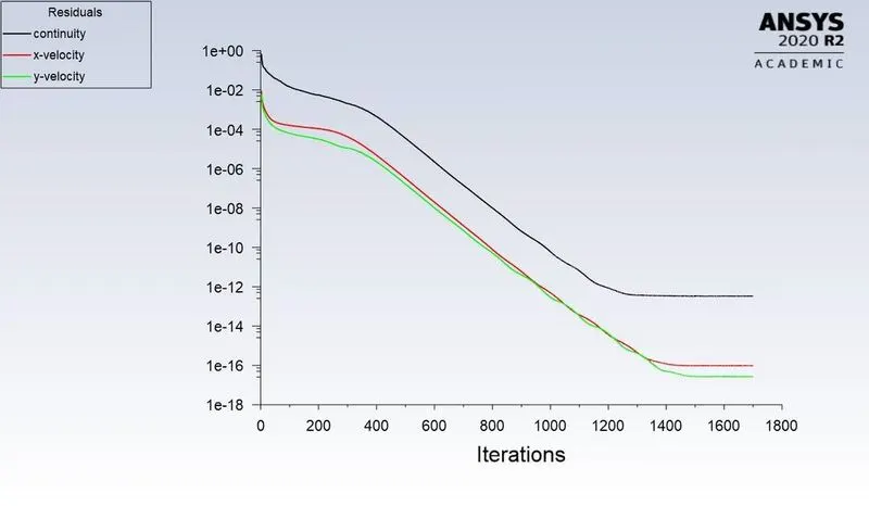
residual plot:

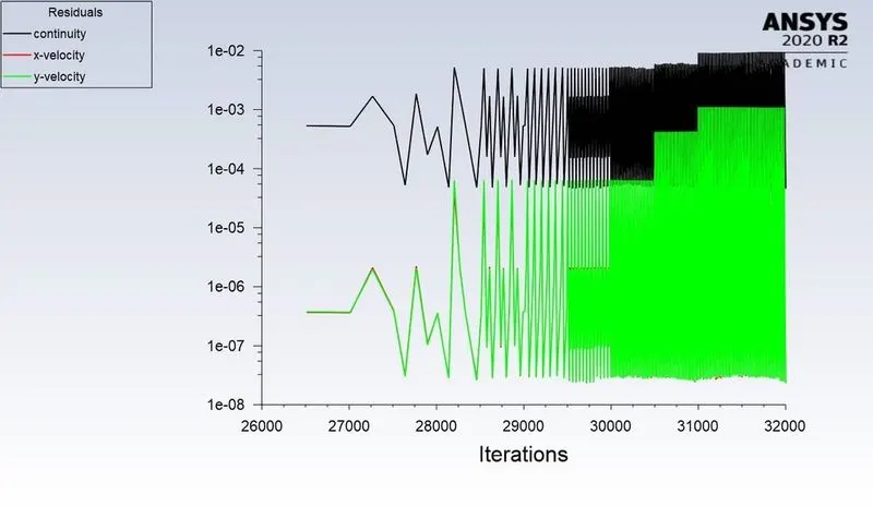
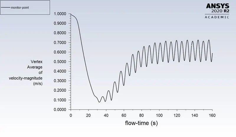
Vertex average at monitor pints:

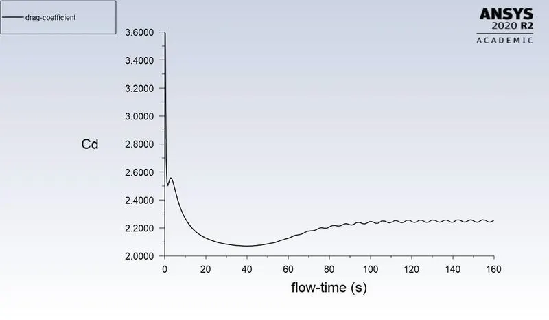
co-efficient of drag at the monitor point walls:

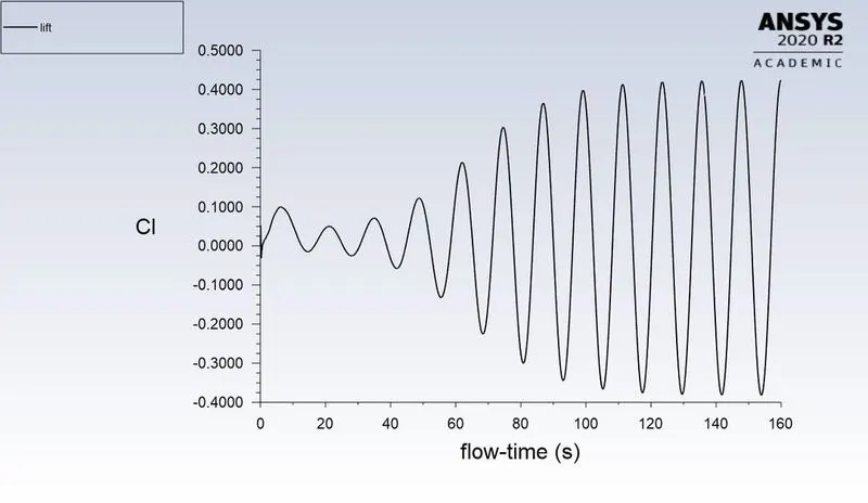
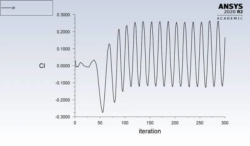
co-efficient of lift at the monitor point:

Velocity and pressure contour plots:

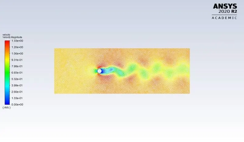
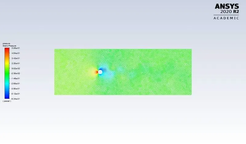
From the contour plot, the stagnation point at the front of the cylinder and the flow separation happening on the surface of the cylinder can be seen

The calculation for Strouhal Number.

St=f.D/v

f=2.5/30 = 0.0833

St=0.83.2/1 = 0.166

Inference:

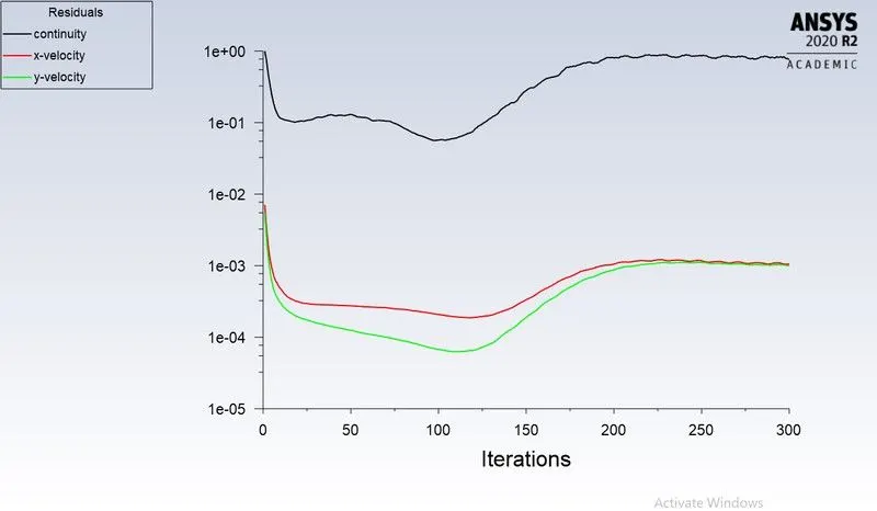
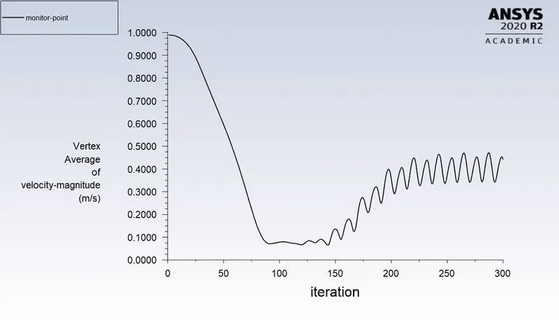
From the Residual plot after 250 iterations the residuals are constant and also from the velocity at the monitor point follows the same pattern hence we can conclude that the solution has reached a steady-state thus there will be no change in the resulting solution even if there is the increase in the number of the solution.

In the simulation using steady-state solver, the results are not time accurate due to which we cannot calculate the Strauhal number whereas in the simulation using unsteady solver the accurate solutions can be obtained from Strauhal number can be calculated which is 0.166.

Part II:

In this part, the simulation is done for the range of Reynolds number by varying the velocity of the flow at the inlet and simulated using steady-state solver.

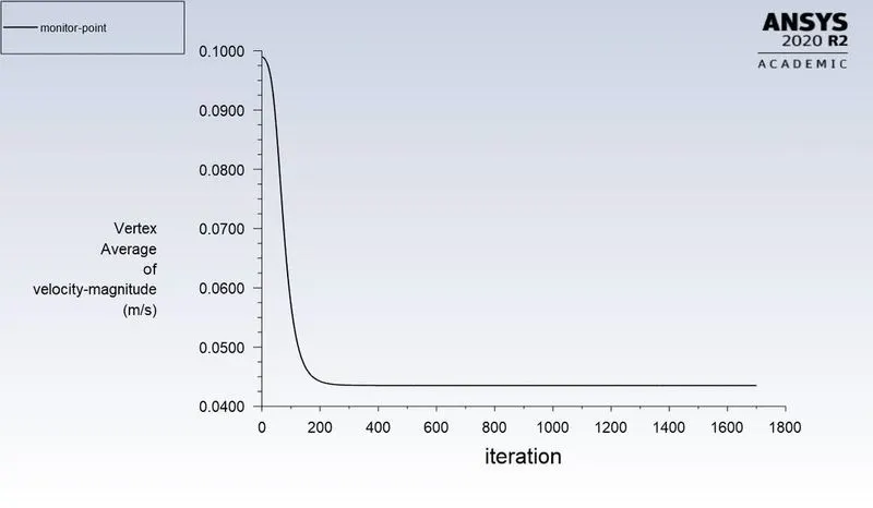
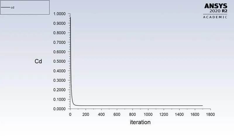
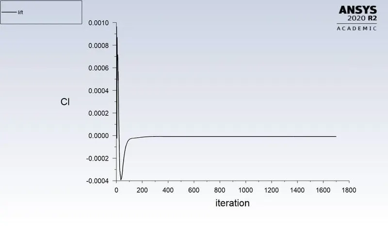
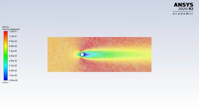
Case 1: Re = 10.

Here Velocity v = 0.1m/s.

Velocity at the monitor point

Coefficient of Drag

Coefficient of lift

Velocity contour plot

Case 2: Re=100

Velocity v = 1m/s

Residual plot:

Velocity at the monitor point.

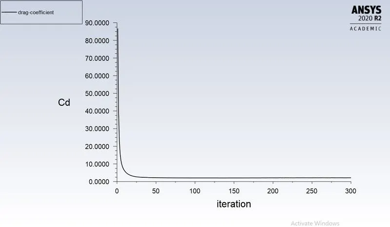
Coefficient of Drag

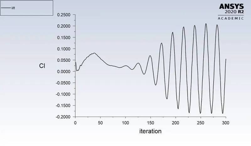
Coefficient of lift

Velocity contour plot

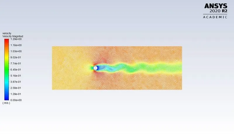
Case 3: Re=1000

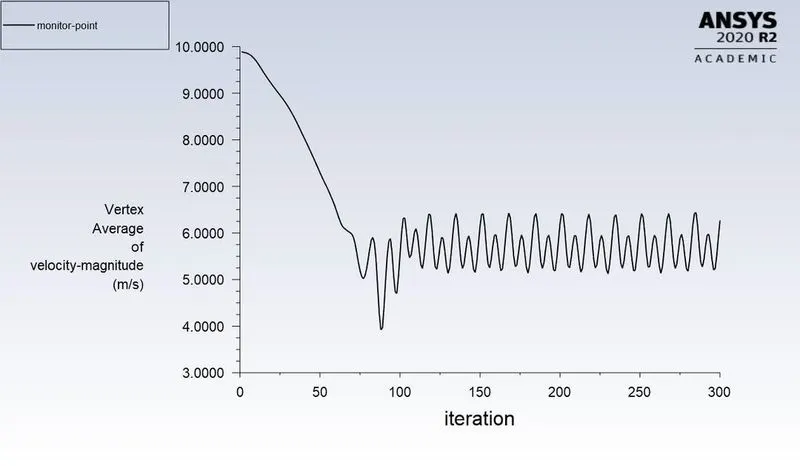
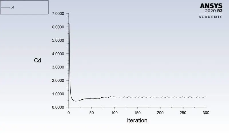
Velocity v = 10m/s

Residual plot:

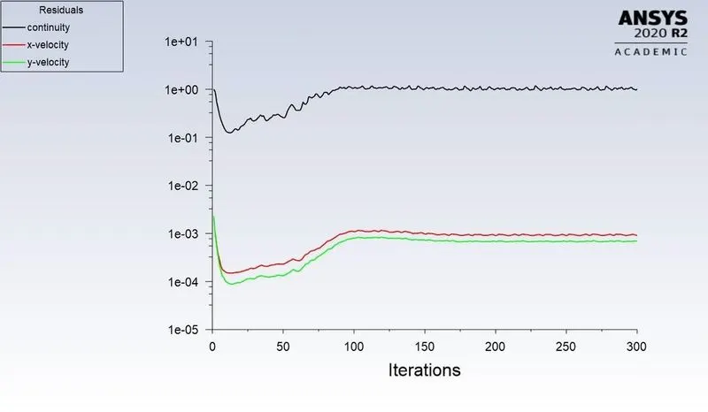
Velocity at the monitor point

Coefficient of Drag

Coefficient of lift

Velocity contour plot

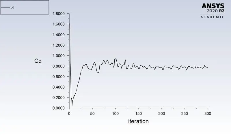
Case 4: Re=10000

Velocity v = 100m/s

Residual plot:

Velocity at the monitor point

Coefficient of Drag

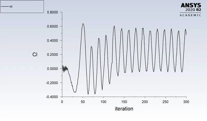
Coefficient of lift

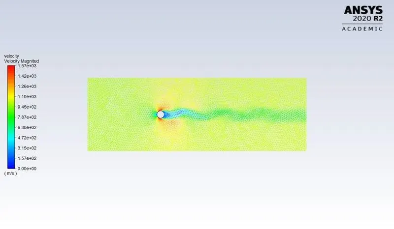
Velocity contour plot

Case 5: Re=100000

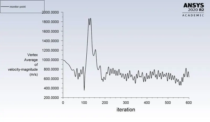
Velocity v = 1000m/s

Residual plot:

Velocity at the monitor point

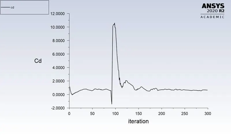
Coefficient of Drag

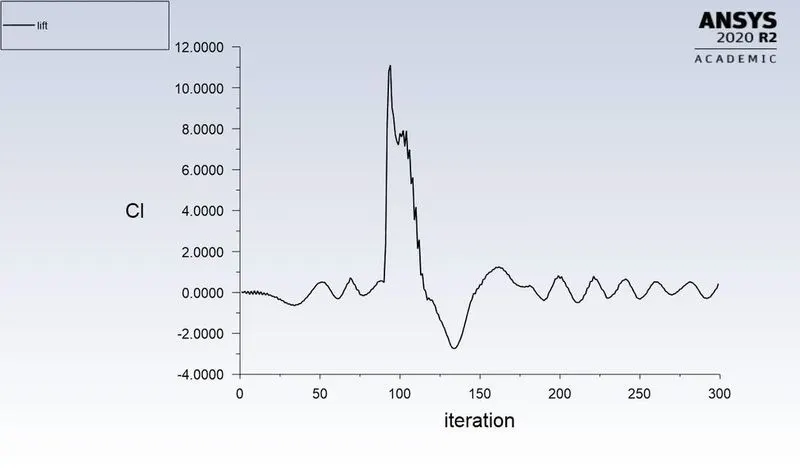
Coefficient of lift

Velocity contour plot

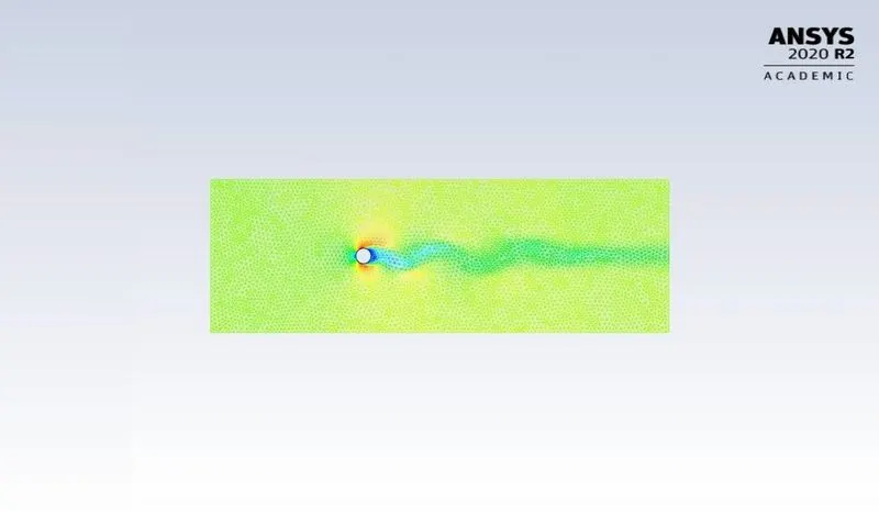
Table depicting the effect of Reynolds number on drag coefficient and lift coefficient.

Velocity in m/s	Reynolds Number	Drag Coefficient
0.1	10	3.3
1	100	1.32
10	1000	0.758
100	10000	0.72
1000	100000	0.62

Conclusion

• When the Reynolds number increases the coefficient of drag decreases. Moreover, when the Reynolds number is large (Re>4000) flow will be turbulent( Chaotic and swirling vortices), in which laminar flow is very small and which leads to lower skin friction drag.
• Firstly, when the velocity increases the coefficient of drag decreases.
• Secondly, for the Reynolds number 10, no vortices can be seen because of low velocity and only boundary layer separation occurred. Also, in low Reynolds number coefficient of drag increases.
• For Reynolds number 100 ( Unsteady state) the vortices can be seen and the shedding frequency calculated. In addition, the value of 0.16 strouhal number is calculated. We have validated this result with experimental data (0.165) where the error appears to be less than 5%.
• In this case, the boundary layer separation decreases there will be less recirculation flow at the wake region behind the cylinder with the reduced drag. All the simulation parameters are kept constant except for the velocity, so increasing the velocity will increase the Reynolds number.
• For the steady case, the flow is not dependent on the time step so strouhal number cannot be calculated for the steady-state but the solution has reached the steady-state after some iterations. We can see vortices for higher Reynolds numbers only.
• For better visualization, we can use contour, vector, and streamline to see the vortex generation when the flow passed over a cylinder.
• In transient case lift coefficient keeps on changing because of the alternate nature of the vortices it never settles down and keeps on repeating the same pattern after some iteration( residual plot). When it comes to steady cases the flow is not dependent on time so the lift coefficient becomes constant after some iterations.

The preferred material for instability:

In order to prevent the unwanted vibration of cylindrical bodies, a longitudinal fin can be fitted on the downstream side, which, provided it is longer than the diameter of the cylinder, will prevent the eddies from interacting, and consequently they remain attached. Obviously, for a tall building, the relative wind could come from any direction. For this reason, helical projections resembling large screw threads are sometimes placed at the top, thereby discouraging the alternate shedding of vortices. Another countermeasure with tall buildings is using variation in the diameter with height, such as tapering - that prevents the entire building from being driven at the same frequency. For example, spiral added to the chimney to avoid vortex shredding