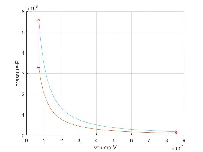
Otto cycle Plot for the pressure and volume

1. Otto cycle is involved with 4 processes adiabatic compression, const volume, adiabatic expansion, and const volume processes.
2. So we are going to give a input variables and their values, and we need to calculate the engine swept-volume, and clearance volume, as per the engine geometric shape.
3. And we need to calculate the P,V, and, T values at all four state points from ideal gas law equation
4. And one more thing we need to calculate the how the volume inside a combustion chamber changes according to the isentropic processes, for that we are going to use a function command which call the parameters at the time of adiabatic compression and expansion processes.

1. In function command we are going to determine the V/VC equation by splitting it into 3 terms,
2. So by copying the engine kinematic function to the we are going to get V compression and expansion values and then from ideal gas law we will get the pressure values,
3. Finally from there we are going to plot the pv diagram, by using plot command

1. And thermal efficiency values by using the formula.
2. all the input variables and equations and their resulting values are plotted by using matlab.
3. the final out come from this experiment is that the thermal efficiency of an otto cycle is96%, with respect to compression ration 12, if the compression ratio value increases then the thermal efficiency may increase but the geometric parameters of an engine may differs.

clear all
close all
clc

% input variables
%p1=initial pressure or atmospheric pressure in bar
%t1=initial temparature in K
%t3= maximumteparature in K

p1=101325;
t1=500;
t3=2300;
%engine geometric parameters
% bore in M
%STROKE in M
%connecting rod in M
% cr= compression ratio 
% gamma= adiabatic process cp/cv=gamma

bore=0.1;
stroke=0.1;
con_rod=0.15;
cr=12;
gamma=1.4;

%calculating the swept volume and the clearence volume

v_swept= pi/4*bore^2*stroke;
v_clearence=v_swept/(cr-1);

% v1,v2= volume in M^3

v1=v_swept+v_clearence;
v2=v_clearence;

%state variables at state point2
% p2*v2^gamma=p1*v1^gamma
%p2= p1*(v2/v1)^gamma
constant_c= p1*v1^gamma;

 V_compression=engine_kinematics(bore,stroke,con_rod,cr,0,180); 
p_compression=constant_c./V_compression.^gamma;

p2=p1*(cr)^gamma;

% p1*v1/t1=p2*v2/t2

t2= p2*v2*t1/(p1*v1);

%state variables at state point3

v3=v2;
% p3*v3/t3=p2*v2/t2
%p3=p2*t3/t2

p3=p2*t3/t2;
constant_c= p3*v3^gamma;

 V_expansion=engine_kinematics(bore,stroke,con_rod,cr,180,0);
 p_expansion=constant_c./V_expansion.^gamma;

%state variables at state point4
v4=v1;
%p4=p3*(v3/v4)^gamma

p4=p3*(v3/v4)^gamma;


for cr=12
    
    otto_cycle_thermal_efficienccy= 1-1/(cr.^gamma-1)
      
          
end

figure(1)
hold on
plot(v1,p1,'*','color','r')
plot(V_compression,p_compression)
plot(v2,p2,'*','color','r')
plot([v2,v3,],[p2,p3])
plot(v3,p3,'*','color','r')
plot(V_expansion,p_expansion)
plot(v4,p4,'*','color','r')
plot([v4,v1],[p4,p1])
xlabel('volume-V')
ylabel('pressure-P')
grid on 



function [V]= engine_kinematics(bore, stroke, con_rod, cr, start_crank, end_crank)

a=stroke/2;
R= con_rod/a;

v_s=pi/4*bore^2*stroke;
v_c=v_s/(cr-1);

% [V/VC= 1+o.5*(cr-1)*[(R+1-cos(theta))-(R^2-sin(theta)^2))^0.5]]

theta= linspace(start_crank,end_crank,180);

term1= 0.5*(cr-1);
term2= R+1-cosd(theta);
term3= (R^2-sind(theta).^2).^0.5;

V = (1+term1*(term2-term3)).*v_c;

end