Week 5.1 - Mid term project - Solving the steady and unsteady 2D heat conduction problem

Objective: we are going to solve the two-dimensional heat conduction for the steady-state and unsteady-states.

For steady-state we are going to use

1. Jacobi
2. gauss-seidel method,
3. successive over relocation methods.

For un-steady state, there will be 2 methods with 3-iterative solvers such as Jacobi, gauss- seidel, sor

For transient state, there will be two scenario’s implicit and explicit for the above same iterative solver methods.

Intro:

Considering general three-dimensional heat conduction we have both time derivative and spatial derivative terms.

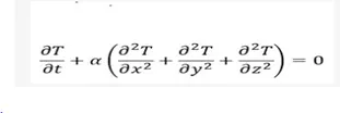
The above equation was a 3-D heat condition where alpha is thermal diffusivity. Now by considering the assumption the above equation is solved for this plate, dimensions in the Z direction are neglected.

The assumption for solving the problem is:

1. Assume that the domain is a unit square.
2. Assume nx=10-ny, for steady-state, and 41 for un-steady, no of points along the x-axis is equal to the no of points along the y-axis.
3. Boundary conditions for the steady and transient cases are taken from the given data in the challenge.
4. And thermal diffusivity (alpha)=1.88e-5 m^2/sec
5. Cfl=alpga*(dt/(dx^2))

Now solving the steady-state equation:

Considering 2-d steady-state equation

(D^2*T/dx^2)+ (d^2*T/d*y)

And here discretizing the equation by applying the central differencing scheme,

clear all
close all
clc

%solving the steady state equation by different iterative solvers
%defining the given inputs
nx=10;
ny=nx;
x=linspace(0,1,nx);
y=linspace(0,1,ny);
dx=x(2)-x(1);
dy=y(2)-y(1);
[xx,yy]=meshgrid(x,y);

%definig the boundary conditions

t=ones(nx,ny);
t(1,:)=900;
t(end,:)=600;
t(:,1)=400;
t(:,end)=800;
told=t;
%eeor_tol,start error
start_error=9e9;
error_tol=1e-4;

dT=1e-2;
alpha=1.88e-5; %thermal siffusivity
%definig the K values
k=2*((dx^2+dy^2)/(dx^2*dy^2));
k1=alpha*(dT/dx^2);
k2=alpha*(dT/dy^2);
% defining the solvers
for iterativ_solver=[1 2 3]
if iterativ_solver==1
  tic;
  t_jacobi=jacobi_iter(start_error,error_tol,xx,yy,nx,ny,dx,dy,t,k,told);
  time_jacobi_in_sec=toc;
elseif iterativ_solver==2
  tic;
  t_gauss=gauss_iter(start_error,error_tol,x,y,nx,ny,dx,dy,k,t,told);
  time_t_gauss_in_sec=toc;
elseif iterativ_solver==3
  tic;
  t_sor=sor_iter(start_error,error_tol,x,y,nx,ny,dx,dy,t,k,told);
  time_t_sor_in_sec=toc;
end
end


function t=jacobi_iter(start_error,error_tol,xx,yy,nx,ny,dx,dy,t,k,told);
  jacobi_iter=1;
  while (start_error > error_tol)
    for i=2:nx-1
      for j=2:ny-1
        term1=(told(i-1,j)+told(i+1,j))/(k*(dx^2));
        term2=(told(i,j-1)+told(i,j+1))/(k*(dy^2));
        t(i,j)=term1+term2;
      endfor
    endfor
    start_error=max(max(abs(told-t)));
    told=t;
    jacobi_iter=jacobi_iter+1;
    figure(1)
    [c,d]=contourf(xx,yy,t);
    colormap(jet)
    colorbar
    title_text=sprintf('jacobi iteration number=%d @steady state',jacobi_iter);
    title(title_text)
    xlabel('x-axis')
    ylabel('u')
    clabel(c,d)
    pause(0.03)
    
  endwhile
  fprintf('no of iteration in jacobi=%d',jacobi_iter);
endfunction


function t=gauss_iter(start_error,error_tol,x,y,nx,ny,dx,dy,k,t,told);
  gauss_iter=1;
  while (start_error>error_tol)
    for i=2:nx-1
      for j=2:ny-1
        t(i,j)=(((t(i-1,j)+told(i+1,j))/dx^2)+((t(i,j-1)+told(i,j+1))/dy^2))/k;
        
      endfor
    endfor
    start_error=max(max(abs(told-t)));
    told=t;
    gauss_iter=gauss_iter+1;
    figure(2);
    [c,d]=contourf(x,y,t);
    colormap(jet)
    colorbar
    title_text=sprintf('GS iteration number=%d @steady state',gauss_iter);
    title(title_text)
    xlabel('x-axis')
    ylabel('u')
    clabel(c,d)
    pause(0.03)
  endwhile
  fprintf('no of iteration in gs iteration=%d',gauss_iter);
endfunction
%

function t=sor_iter(start_error,error_tol,x,y,nx,ny,dx,dy,t,k,told);
  sor_iter=1;
  omega=1.2;
  while (start_error>error_tol);
    for i=2:nx-1
      for j=2:ny-1
        t_gs=(((t(i-1,j)+told(i+1,j))/dx^2)+((t(i,j-1)+told(i,j+1))/dy^2))/k;
        t(i,j)=omega*(t_gs)+(1-omega)*(told(i,j));
end
end
start_error=max(max(abs(told-t)));
    told=t;
    sor_iter=sor_iter+1;
    sor=figure(3)
    [c,d]=contourf(x,y,t);
    colormap(jet)
    colorbar
    title_text=sprintf('sor iteration number=%d @steady state',sor_iter);
    title(title_text)
    xlabel('x-axis')
    ylabel('u')
    clabel(c,d)
    pause(0.03) 
end
fprintf('no of iteration in sor=%d',sor_iter);    
  
endfunction
%

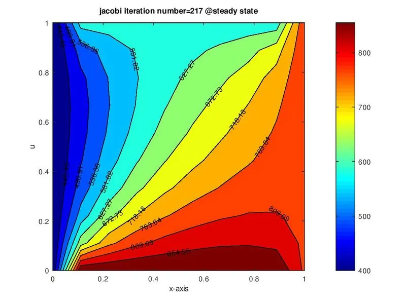
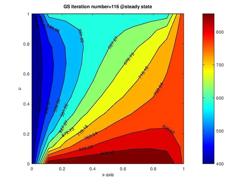
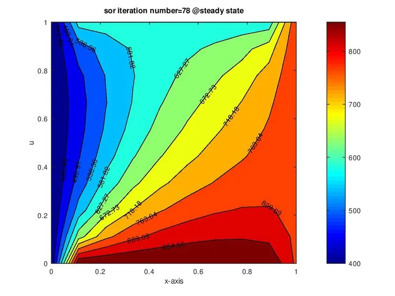
Conclusion:

From the above plots it can be inferred that the sor method takes less time and less no of iteration when compared to the other two iteration methods. Therefore SOR will give fast and well results compare with others.

Now we are going to solve the transient state equation methods:

Transient state 2D state heat condition equation is solved in both ways such are explicit and implicit methods.

D*T*t/d+alpha(d^2*T/d*x^2+d^2*T/d*y^2)=0

Solving the above equation explicitly:

The explicit approach is used in numerical analysis for obtaining numerical approximation s to the ere solution of time-dependent ordinary or partial differential equations are required in computer simulations of a physical process. These are calculated the state of a system at a later time from the state of the system at the current time.

In this method, each differential equation approach contains only one unknown and can be solved explicitly for this one unknown using method.

Here this equation time derivative terms are calculated using the 1^st order differential equation and whereas the 2 has 2^nd order derivative terms and elliptical in nature so information needs to be taken from all the points equally, so, a central differencing scheme is applied for the discretizing terms 2.

The discretized equation for 2d heat condition equation for the explicit as follows:

Solving the transient state in implicitly:

The implicit approach is used in numerical analysis for obtaining numerical approximations to the solution of time-dependent ordinary or partial differential equations as in computer simulations’

Implicit methods find the solution by solving an equation involving both the current and next state of the system. Mathematically if y (t) is the current system and y(t+dt) is the state at the later time dt, then, for an explicit method y(t+dt)=f(y(t)).

Hence in this equation time derivative terms are calculated using the first-order derivative terms and elliptical in nature so information needs to be taken from all the points equally,i.e. a central differencing scheme is applied for the desecrating the term2.

The final discretized equation for 2-d heat conduction equation for the implicit form is as follows.

The equation is solved iteratively using different iterative methods such as Jacobi, gauss-sedial,sor methods.

In Jacobi, the unknowns on the right-hand side are assumed to have an initial value i.e t at ‘n+1’ at all nodes is assumed. Using the equation, then the LHS is calculated. On the next value of I,j same method is followed to calculate lhs, thus in the first iteration valued of t for time ‘n+1,’, is calculated at all nodes. The difference between t at ‘n+1, was obtained and t at ‘n+1’ which was assumed as previously taken. If it Is greater than a specified tolerance value, iteration is carried out to calculate t at ‘n+1’. But in the second iteration, t at ‘n+1’, is assumed as the value of t which was obtained in the previous iteration.

Once the value of t is found iteratively whose error is less than the tolerance value, the value of t is calculated at the next time step n+2 using the same steps.

Equation for Jacobi:

term1=(1+(2*k1)+(2*k2))^(-1);

term2=k1*term1;

term3=k2*term1;

h=(told(i-1,j)+told(i+1,j));

v=(told(i,j-1)+told(i,j+1));

t(i,j)=(to(i,j)*term1)+term2*h+term3*v;

the gauss-seidel method is similar to the Jacobi method, but the only difference is for the first iteration when the value of t at a particular node is calculated. This updated value at that node is used to calculate the value at the next node. But the error term is calculated similarly to the Jacobi method, i.e t at ‘n+1’, calculated minus the t at ‘n+1’ previous one.

Once the value of t is found iteratively whose error is less than the tolerance value, the value of t is calculated at the next time step ‘n+2’ using the same method.

Equation for gauss-seidel are

term1=(1+(2*k1)+(2*k2))^-1;

term2=k1*term1;

term3=k2*term1;

h=(t(i-1,j)+told(i+1,j));

v=(t(i,j-1)+told(i,j+1));

t(i,j)=to(i,j)*term1+term2*h+term3*v;

SOR method:

This can be applied either by using Jacobi or gauss but the only difference is considered here called omega(scaling factor) which in turn makes the process faster by which the number of iterations required to solve will be minimum

The optimum vale of omega is calculated by using the formula=omega=2/(1+sin(pi*dx))

Equation for SOR:

term1=(1+(2*k1)+(2*k2))^-1;

term2=k1*term1;

term3=k2*term1;

h=(t(i-1,j)+told(i+1,j));

v=(t(i,j-1)+told(i,j+1));

t(i,j)=omega*(to(i,j)*term1+term2*h+term3*v)+(1-omega)*to(i,j);

clear all
close all
clc

% defining the inputs
nx=10;
ny=nx;
l=1
x=linspace(0,1,nx);
y=linspace(0,1,ny);
dx=x(2)-x(1);
dy=y(2)-y(1);
dt=0.01;
alpha=1.88e-5; %thermal diffusivity
[xx,yy]=meshgrid(x,y);
%defining the boundary condition

t=298*ones(nx,ny);
t(1,:)=900;
t(end,:)=600;
t(:,1)=400;
t(:,end)=800;
%rounding off the corner values by taking the avg value
t(1,1)=(400+900)/2;
t(1,ny)=(900+800)/2;
t(nx,1)=(400+600)/2;
t(nx,ny)=(600+800)/2;
told=t;
to=told;
%error tol,start error
error_tol=1e-4;
start_error=9e9;
k1=(alpha*dt)/(dx^2);
k2=(alpha*dt)/(dy^2);
omega=2/(1+sin(pi*dx));
CFL=(alpha*dt)/(dx^2);
%explicit approch
iter_method=1
if iter_method==1
  time=explicit_jacobi(nx,ny,xx,yy,t,k1,k2,told);
end
%

%defining the solvers
%unstudy state or transient state
%implicit state approch

for iter_method=[1 2 3]
  if iter_method==1
    time=implicit_jacobi(error_tol,nx,ny,xx,yy,t,k1,k2,told,to);
  elseif iter_method==2
    time=implicit_gauss_sedial(error_tol,nx,ny,xx,yy,t,k1,k2,told,to);
  elseif iter_method==3
    time=implicit_sor(error_tol,xx,yy,nx,ny,t,k1,k2,told,to,omega);
 

  endif
 endfor
%

function [out]=explicit_jacobi(nx,ny,xx,yy,t,k1,k2,told);
  % explit jacobi method for transient state
  
  jacobi_iter=1
 tic
 for m=1:12000
       for i=2:nx-1
      for j=2:ny-1
        term1=told(i,j);
        term2=k1*(told(i+1,j)-2*told(i,j)+told(i-1,j));
        term3=k2*(told(i,j+1)-2*told(i,j)+told(i,j-1));
        t(i,j)=term1+term2+term3;
    end
    end
    start_error=max(max(abs(told-t)));
    told=t;
    jacobi_iter=jacobi_iter+1;
    

end
iter_time=toc
  figure(7)
    [c,d]=contourf(xx,yy,t);
    colormap(jet)
    colorbar
    title_text=sprintf('jacobi iteration number=%d @un-steady state explicit',jacobi_iter);
    title(title_text)
    xlabel('x-axis')
    ylabel('u')
    clabel(c,d)
    pause(0.03)
    out=iter_time;
endfunction
%

function t=implicit_jacobi(error_tol,nx,ny,xx,yy,t,k1,k2,told,to);
  %implicit jacobi method for transient state
  
   
  jacobi_iter=1;
  tic
  for m=1:12000 % time loop
    start_error=9e9;
    while(start_error>error_tol) %convergence loop
    for i=2:nx-1 %nodal loop
      for j=2:ny-1
        term1=(1+(2*k1)+(2*k2))^(-1);
        term2=k1*term1;
        term3=k2*term1;
        h=(told(i-1,j)+told(i+1,j));
        v=(told(i,j-1)+told(i,j+1));
        t(i,j)=(to(i,j)*term1)+term2*h+term3*v;
        
      end
    end
    start_error=max(max(abs(told-t)));
    told=t;
    jacobi_iter=jacobi_iter+1;
    
  end
to=t;
end
iter_time=toc
figure(4)
    [c,d]=contourf(xx,yy,t,'ShowText','on');
    colormap(jet)
    colorbar
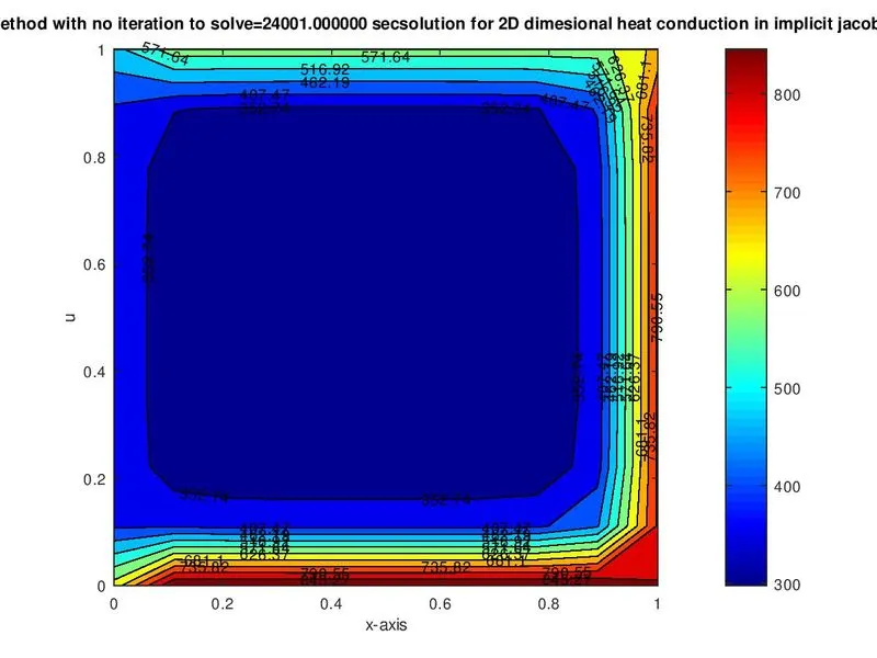
    title_text=sprintf('solution for 2D dimesional heat conduction in implicit jacobi method with no iteration to solve=%f sec',jacobi_iter,iter_time);
    title(title_text)
    xlabel('x-axis')
    ylabel('u')
    clabel(c,d)
    pause(0.03)
    fprintf('no of iteration in jacobi=%d and time in sec=%f',jacobi_iter,iter_time);
    
endfunction
%

function t=implicit_gauss_sedial(error_tol,nx,ny,xx,yy,t,k1,k2,told,to);
  % implicit gauss sediaal transient state
  
  gs_iter=1;
  tic
  for m=1:12000
    start_error=9e9;
    while(start_error>error_tol)
    for i=2:nx-1
      for j=2:ny-1
        term1=(1+(2*k1)+(2*k2))^-1;
        term2=k1*term1;
        term3=k2*term1;
        h=(t(i-1,j)+told(i+1,j));
        v=(t(i,j-1)+told(i,j+1));
        t(i,j)=to(i,j)*term1+term2*h+term3*v;
      end
    end
    start_error=max(max(abs(told-t)));
    told=t;
    gs_iter=gs_iter+1;
  end
  to=t;
endfor
iter_time=toc
figure(5)
    [c,d]=contourf(xx,yy,t,'ShowText','on');
    colormap(jet)
    colorbar
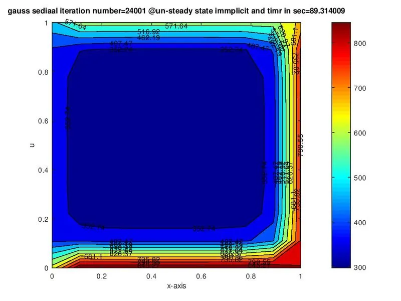
    title_text=sprintf('gauss sediaal iteration number=%d @un-steady state immplicit and timr in sec=%f',gs_iter,iter_time);
    title(title_text)
    xlabel('x-axis')
    ylabel('u')
    clabel(c,d)
    pause(0.03)
    fprintf('no of iterration in GS=%d and timr in sec=%f',gs_iter,iter_time);
    
endfunction
%

function t=implicit_sor(error_tol,xx,yy,nx,ny,t,k1,k2,told,to,omega);
  % implicit sor method for transient state
  
  sor_iter=1;
  tic
  for m=1:12000
    start_error=9e9;
    while(start_error>error_tol)
    for i=2:nx-1
      for j=2:ny-1
        term1=(1+(2*k1)+(2*k2))^-1;
        term2=k1*term1;
        term3=k2*term1;
        h=(t(i-1,j)+told(i+1,j));
        v=(t(i,j-1)+told(i,j+1));
        t(i,j)=omega*(to(i,j)*term1+term2*h+term3*v)+(1-omega)*to(i,j);
      end
    end
    start_error=max(max(abs(told-t)));
    told=t;
    sor_iter=sor_iter+1;
   
  endwhile
  to=t;
endfor
iter_time=toc
figure(6)
    [c,d]=contourf(xx,yy,t);
    colormap(jet)
    colorbar
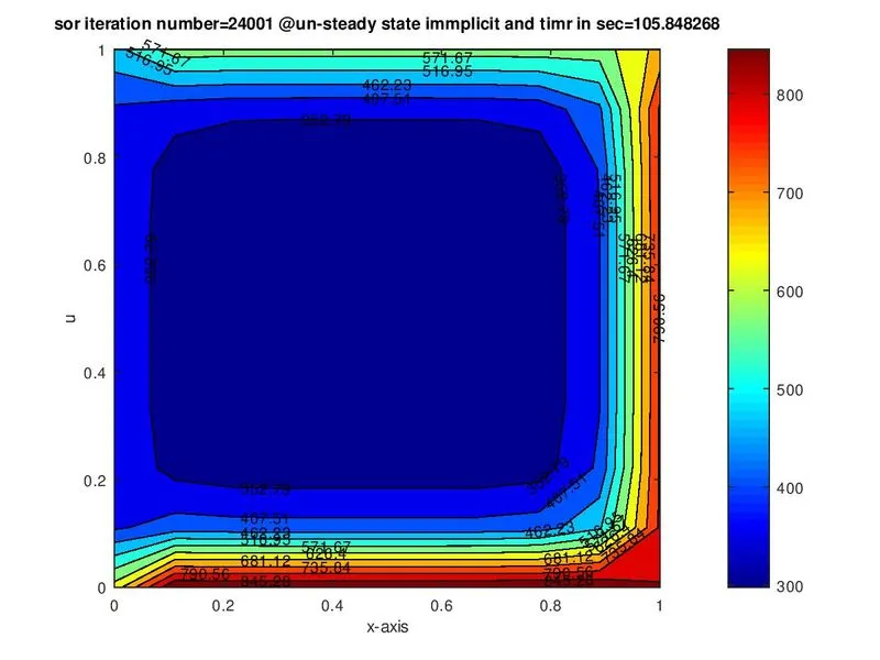
    title_text=sprintf('sor iteration number=%d @un-steady state immplicit and timr in sec=%f',sor_iter,iter_time);
    title(title_text)
    xlabel('x-axis')
    ylabel('u')
    clabel(c,d)
    pause(0.03)
    fprintf('no of iterration in sor=%d and timr in sec=%f',sor_iter,iter_time);
endfunction

\

Conclusions:

I conclude the above heat conduction processes or methods are as in steady-state equation SOR method yields the result value very quickly when compared to other two methods, whereas Jacobi method takes more no of iteration and more no of time to solve the unknowns.it is recommend

So the SOR method is most efficient when compared to the other two methods to solve the steady-state equation.

2. For transient equations, the time required to solve is more when compared to steady-state equations, so it is better to solve the2-d heat conduction equation with steady-state conditions.

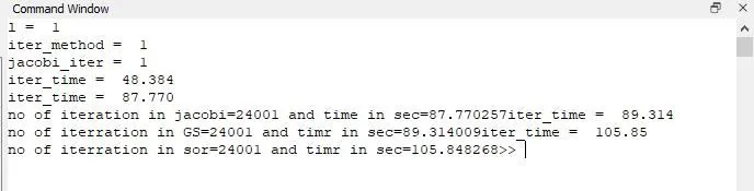
In un-steady state equation, explicit methods yield the result quickly when compared to the implicit method, but it is better under the value f CFL is less than 0.25

When the transient state equation is solved implicitly Jacobi takes less time when compared to the other two methods whereas SOR is more stable compared to other methods.