Week 4 - CHT Analysis on Exhaust port
CHT ANALYSIS ON EXHAUST MANIFOLD
1) What is CHT Analysis, Why and Where it is used?
Conjugate Heat Transfer (CHT) refers to the coupling of conduction in solids with the convective and radiative heat transfer in the surrounding fluids. In other words, CHT corresponds with the combination of heat transfer in solids and heat transfer in fluids. In solids, conduction often dominates whereas, in fluids, convection usually dominates. Efficiently combining heat transfer in fluids and solids is the key to designing effective heaters, coolers, or heat exchangers. Heat transfer in solids and heat transfer in fluids are combined in the majority of applications. This is because fluids flow around the solids, or between solid walls, and because solids are usually immersed in a fluid.
The CHT Analysis is used in processes that involve variations of temperature within solids and fluids, due to thermal interaction between the solids and fluids. The exchange of thermal energy between the two physical bodies is called the study of Heat Transfer, the rate of transferred heat is directly proportional to the temperature difference between the bodies. A typical example is the heating or cooling of a solid object by the flow of air in which it is immersed.
The physics of conjugate heat transfer is common in many engineering applications, including heat exchangers, HVAC, and electronic component design.
2)CHT ANALYSIS ON EXHAUST MANIFOLD
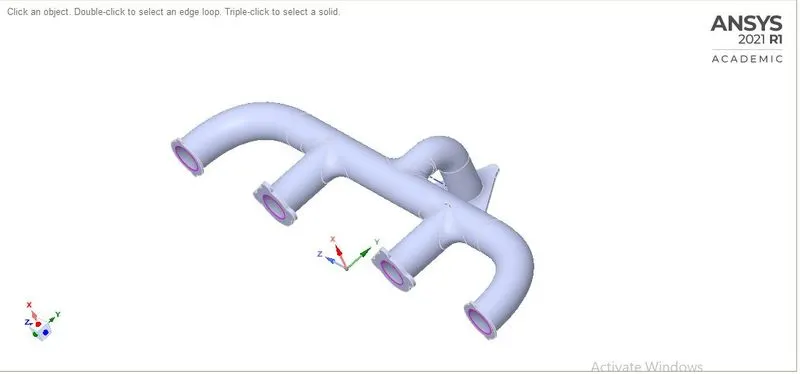
The figure below shows the Exhaust Manifold of a 4 cylinder engine.
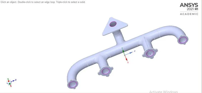
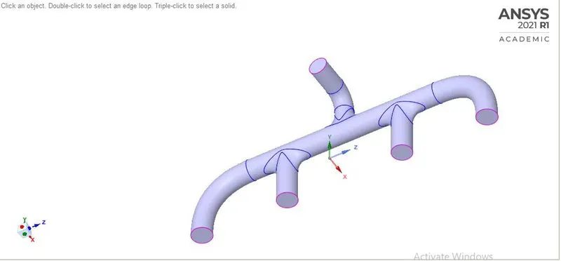
First, the geometry is prepared using the volume extract tool, i.e the fluid volume is extracted. The image below shows solid and fluid volumes.
Solid Volume:-
Fluid Volume:-
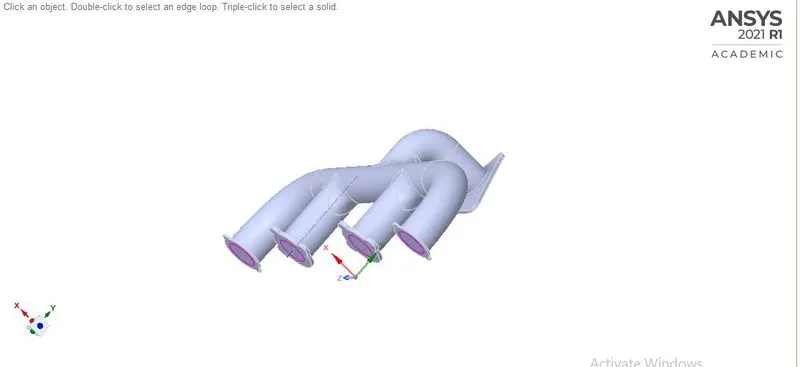
Now using share topology in order to have conformal mesh between the solid and fluid volume.
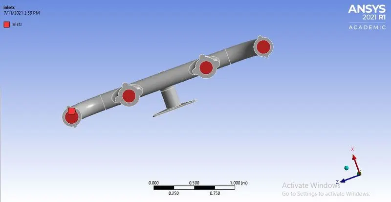
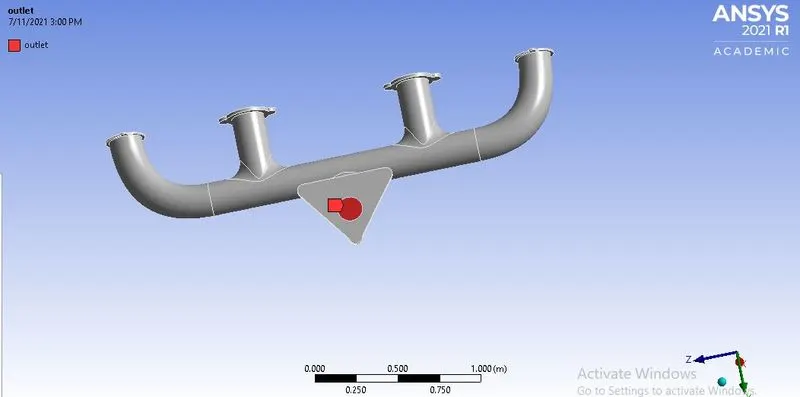
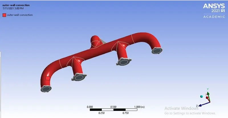
Named selections given to the geometry are as follows:
Inlet:-
Outlet:-
Outer Wall:-
THE PROBLEM IS SOLVED USING TWO CASES, ONE HAVING BASELINE MESH AND ANOTHER ONE WITH REFINED MESH.
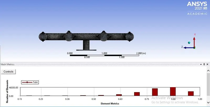
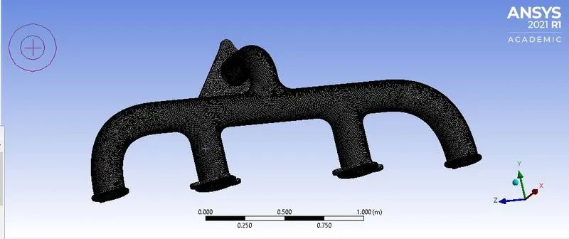
CASE 1) In this case the mesh is a baseline with elements of about 136990.
BASELINE MESH:-
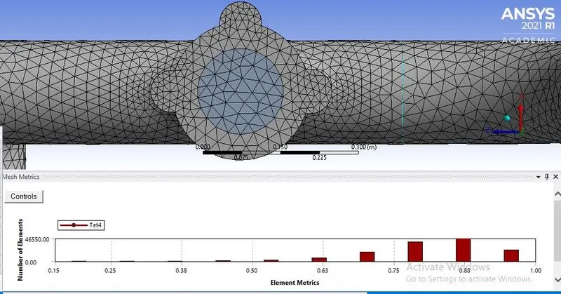
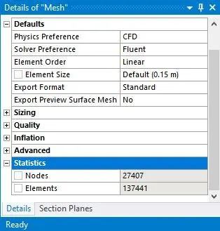
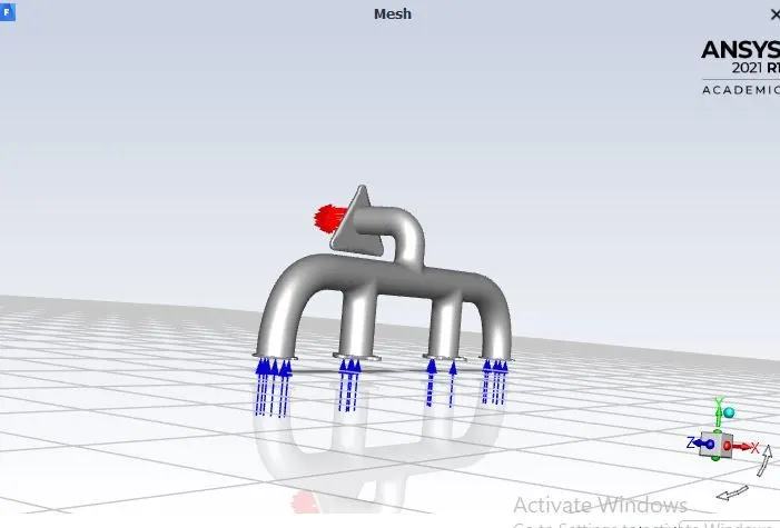
after completing the mesh processes we will open the setup page the initial modeling will look like this:
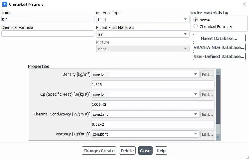
Material: The material selected for solid is aluminum and for fluid is air.
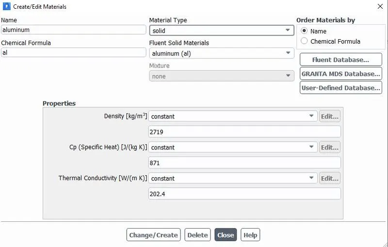
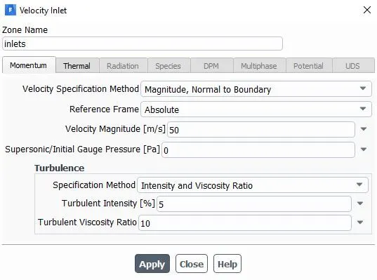
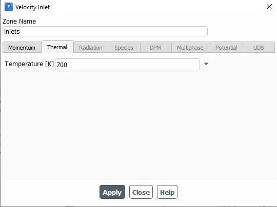
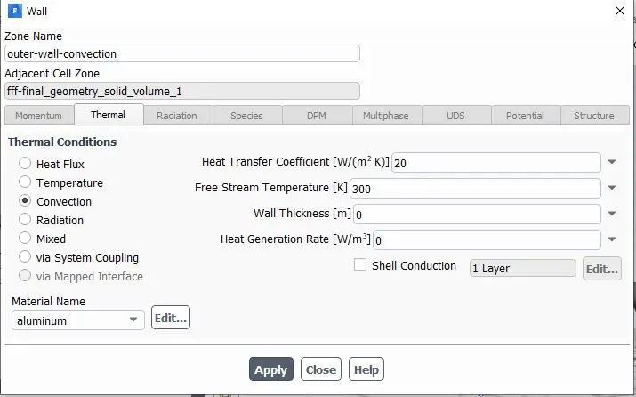
Boundary conditions: The boundary conditions given at different selections are as follows:
Inlet:
Outer Wall:
outlet:
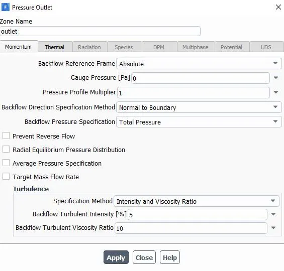
then doing all these steps we are gonna do the initialization then we also going to create an animation result by running with 150 iterations
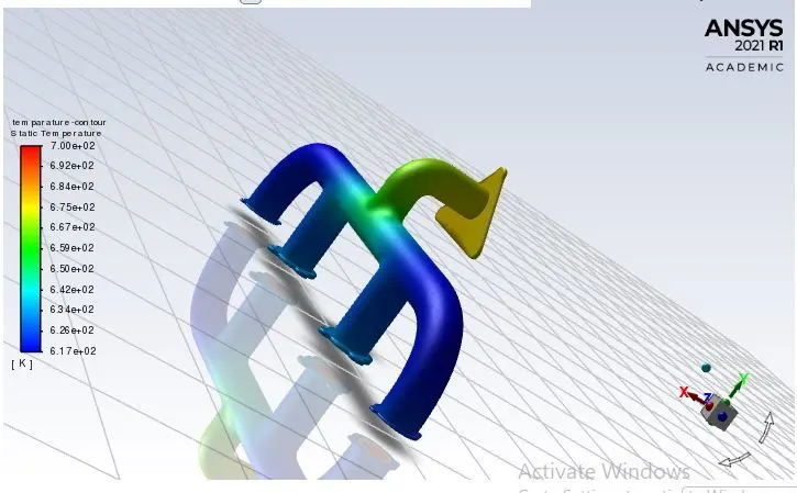
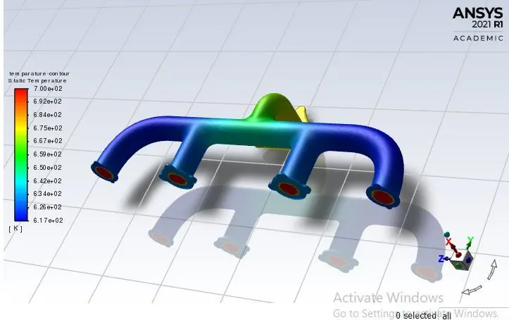
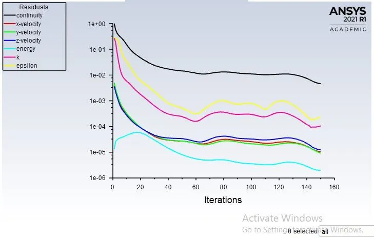
Results: Solving the problem for about 150 iterations, the results are as follows:
residual plot:
Post Processing :
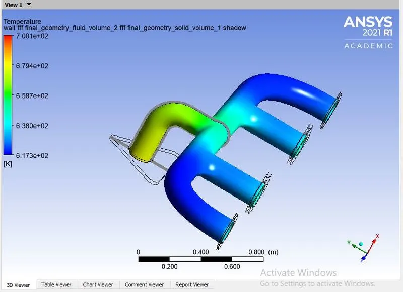
The temperature at the outer wall is shown in the image below. It can be seen that the temperature at the outer wall at the inlet is low as compared to that of at the outlet, this is because the velocity is lower at the inlets as compared to that at the outlet. So as the velocity increases, Reynold's number increases, and the heat transfer coefficient also increase thus increasing the transfer of heat from the fluid to the solid.
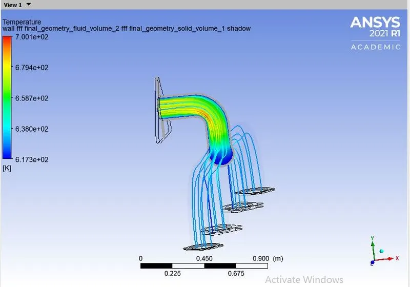
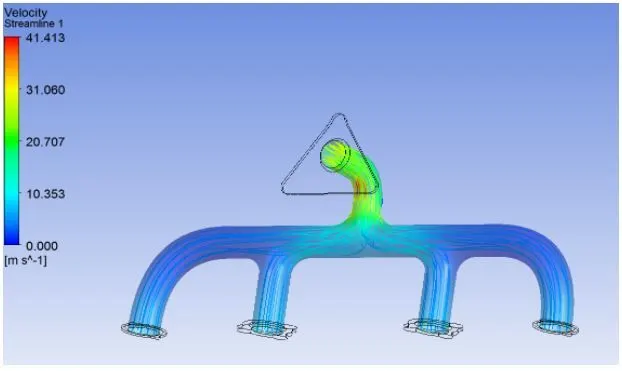
Velocity streamline: The Velocity streamline starting from the inlets is shown in the image below. Here we can see that the velocity is low in the inlet sections (the 4 inlets) whereas the velocity is higher at the outlet section, this is because of mass conservation. There are four inlets and only one outlet, all the faces are of same size i.e the area is same; and area times velocity is the flow rate.
A1V1 + A2V2 + A3V3 + A4V4 = A5V5
where, A1, A2,A3,A4 are the areas at inlet 1,2,3,4 respectively and A5 is the area at outlet
V1,V2,V3,V4 are the velocities at inlet 1,2,3,4 respectivelt and V5 is the velocity at outlet.
As A1=A2=A3=A4=A5,
Therefore
V1 + V2 + V3 + V4 = V5
Hence velocity at the outlet is higher than that at the inlets.
Wall Heat Transfer Coefficient Plot:-
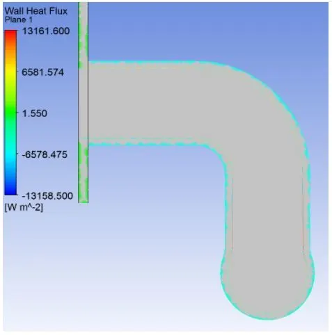
Wall heat transfer coefficient is a quantity that is calculated only at the wall that is adjacent to the fluid.
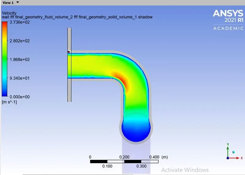
Velocity Plot:-
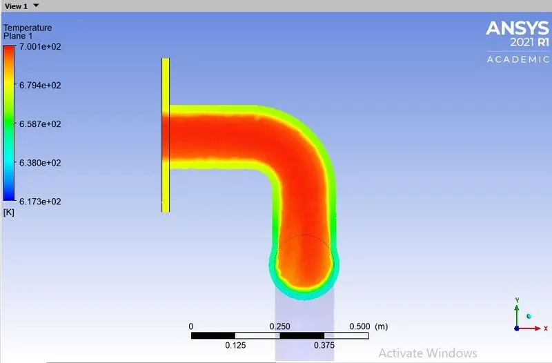
Temperature Plot:-
CASE 2)
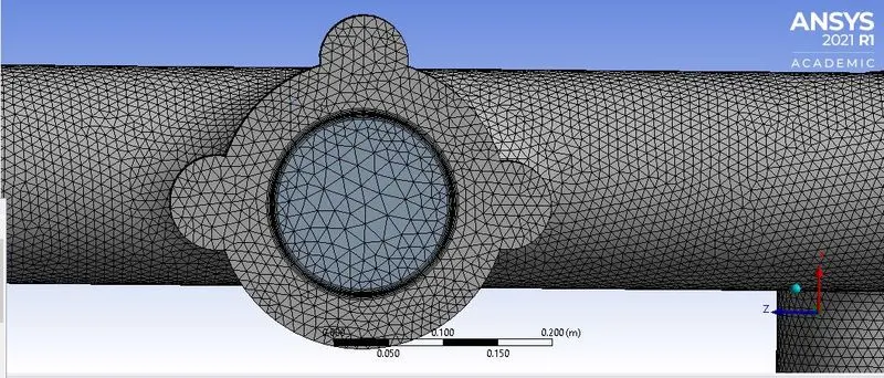
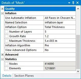
In this case, the mesh is finer at the solid part, having elements of about 1185562. Also, 5 inflation layers are provided with a growth rate of 1.2 and a maximum thickness of 5 e-003 m.
RESULTS: Solving the problem for about 150 iterations, the results are as follows:
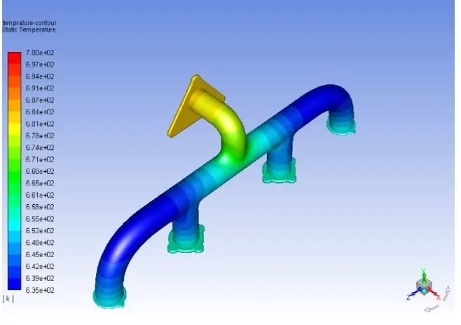
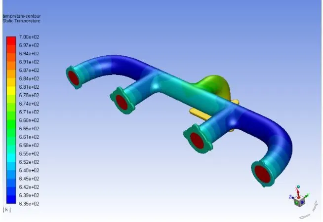
Post Processing:
Temperature at wall
Velocity streamline:
Wall heat transfer coefficient plot:
Velocity plot:
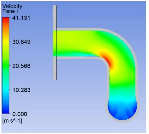
Temperature plot:
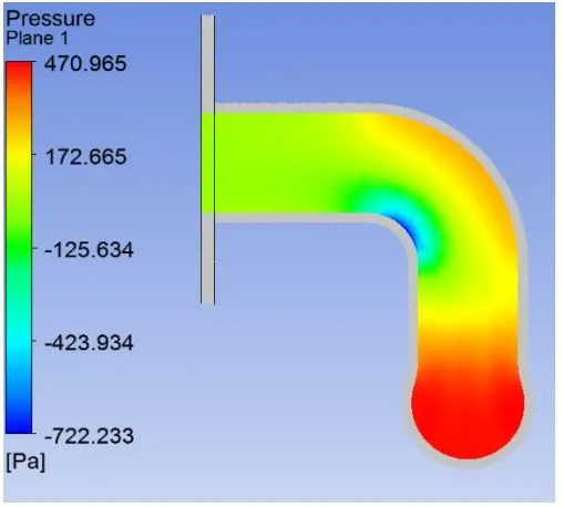
Pressure plot:
DOES REFINING THE MESH PRODUCED ANY CHANGES TO THE RESULT?
In order to find what changes are produced by refining the mesh, the following comparisons are made between the different quantities viz. Wall heat transfer coefficient, Velocity, and Temperature of baseline mesh and refined mesh (Left figure represents the respective quantity of baseline mesh whereas the right one indicates the respective quantity of the refined mesh.)
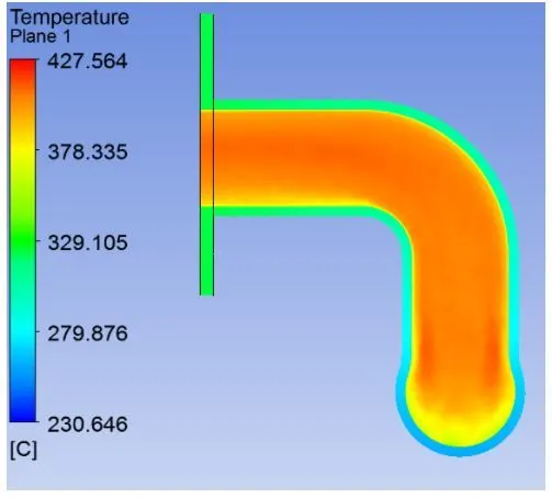
It can be seen from the images below that by refining the mesh and adding the inflation layers we get a smooth plot at the inner boundary. We know that the heat transfer coefficient is only available in the first cell that is attached to the wall which can be seen properly in the refined mesh image.
Also, the values of wall heat transfer coefficient, velocity, and temperature are seen to be increased in the refined case (right-side images) as compared to that in the base mesh (left-side images).
3) How would you verify if the HTC predictions from the simulations are right? On what factors does the accuracy of the prediction depend?
Nusselt's number is given by:-
Nu=h⋅L/K
therefore, h=Nu⋅K/L
where h= Heat Transfer Coefficient
Nu= Nusselt's Number
K= Thermal conductivity coefficient
L= Characteristic Length
We know that Nusselt's number is a function of Reynold's number, which in turn is a function of flow velocity
Therefore, HTC is directly proportional to flow velocity.
We can see from the images above that both the HTC and velocity are maximum near the outlet.
Hence, the HTC predictions from the simulations are correct.
Factors affecting the prediction are as follows:-
- Element Size and Quality = The finer the mesh, the accurate the results.
- Inflation Layer = It increases the quality of mesh near the boundary interface and helps to capture smooth plots of different quantities.
- Mesh at the solid-fluid interface = The mesh at the solid-fluid interface must be conformal.