Week 3 - Solving second order ODEs

Aim: To simulate the motion of simple pendulum by solvind 2nd order differential equation using python considering damping coefffcient.

Objective: 1)To Understand the concept of converting 2nd order ODE to first order linear system.

2) To understand the odeint function to solve the diffential equation when provided with function and its derivative.

Equation for motion of simple pendulum:

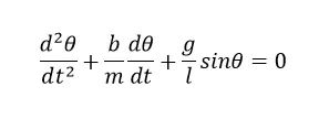
To convert 2nd order ode to 1st order ode

consider, θ=θ1(displacement),

dθ/dt=dθ1/dt=θ2(velocity)

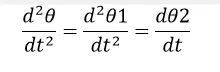
substituting the above in our 2nd order ode

we get,

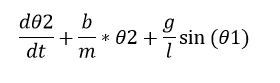
The above equation is linear and can be solved using python

Differential equations are solved in Python with the Scipy.integrate package using function odeint

theta=odeint(model1,theta_0,t, args = (b,m,g,l))

model1 = Function name that returns derivative values at requested θ and t values as dθ/dt

theta_0=initial values angular displavement and velocit in our case

t=Time points at which the solution should be reported.

args()= Allows additional information to be passed into the model function.The args input is a tuple sequence of values.

Code:

import math
import numpy as np
from scipy.integrate import odeint
import matplotlib.pyplot as plt

def model1(theta,t,b,m,g,l):
	theta1=theta[0]
	theta2=theta[1]
	theta1_dt=theta2
	theta2_dt=-(b/m)*theta2-(g/l)*math.sin(theta1)
	dtheta_dt=[theta1_dt,theta2_dt]
	return dtheta_dt
b=0.05
g=9.81
l=1
m=1

#initial condition
theta_0=[0,3]
#time step
t=np.linspace(0,20,150)
#solve ode
theta=odeint(model1,theta_0,t, args = (b,m,g,l))

print(theta)
plt.plot(t,theta[:,0],'blue',label=r'$\frac{d\theta_1}{dt}=\theta2$')
plt.plot(t,theta[:,1],'red',label=r'$\frac{d\theta2}{dt}=-\frac{b}{m}\theta_2-\frac{g}{l}sin\theta_1$')
plt.legend(loc='best')
plt.show()
#animation and ploting
ct=1
displacement=theta[:,0]
for i in displacement:
	x0=0
	y0=0
	x1=l*math.sin(i)
	y1=-l*math.cos(i)

	#plotting
	plt.figure()
	# point of attachment of string
	plt.plot([-1.5,1.5],[0,0],linewidth=9)
	#rope of pendulum
	plt.plot([x0,x1],[y0,y1],linewidth=5)
	#bob of pendulum
	plt.plot(x1,y1,'-o',markersize=20)
	plt.xlim=([-1.5,1.5])
	plt.ylim=([-1.5,0.5])
	filename='test%05d.png'%ct
	plt.savefig(filename)
	ct=ct+1

Plot:

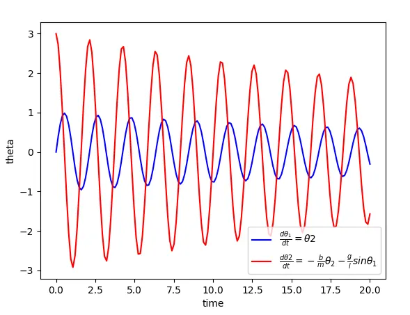
The angular displacemet starts from 0 as we have provided the input, while the angular velocity starts at 3m/s. Both velocity and displacement are changing sinusoidal function whose amplitude approaches zero as time increases as we have considered damp factor in our equation.

Animation:

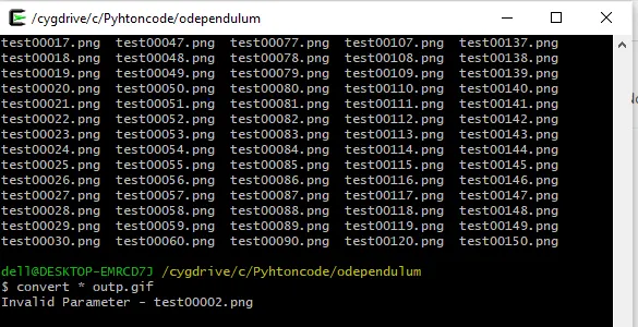
Errors: No major errors faced in program, but error with cygwin to create animation was consistent.