Solving second order ODEs using MATLAB
Solving second order ODEs
OBJECTIVE:
We have to
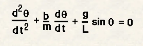
- write a program that solves the following ODE. This ODE represents the equation of motion of a simple pendulum with damping
- animate the motion of the pendulum
THEORY:
The Simple Pendulum
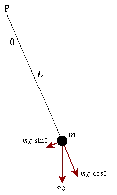
A simple pendulum consists of a mass m hanging from a string of length L and fixed at a pivot point P. When displaced to an initial angle and released, the pendulum will swing back and forth with periodic motion. By applying Newton's second law for rotational systems, the equation of motion for the pendulum may be obtained

and rearranged as

If the amplitude of angular displacement is small enough that the small angle approximation () holds true, then the equation of motion reduces to the equation of simple harmonic motion

The simple harmonic solution is

with being the natural frequency of the motion.
The Real (Nonlinear) Pendulum
When the angular displacement amplitude of the pendulum is large enough that the small angle approximation no longer holds, then the equation of motion must remain in its nonlinear form
This differential equation does not have a closed form solution, and must be solved numerically using a computer. Mathematica numerically solves this differential equation very easily with the built in function NDSolve[ ].
Small Initial Amplitude
The small angle approximation is valid for initial angular displacements of about 20° or less. The (0.132MB) mpeg movie at left shows two pendula: the black pendulum assumes the linear small angle approximation of simple harmonic motion, the grey pendulum (hidded behind the black one) shows the numerical solution of the actual nonlinear differential equation of motion. For small initial angular displacements the error in the small angle approximation becomes evident only after several oscillations.
Large Initial Amplitude
When the initial angular displacement is significantly large that the small angle approximation is no longer valid, the error between the simple harmonic solution and the actual solution becomes apparent almost immediately, and grows as time progresses. In the (0.226MB) mpeg move at left, the dark blue pendulum is the simple approximation, and the light blue pendulum (initially hidden behind the dark blue one) shows the numerical solution of the nonlinear differential equation of motion
PROBLEM STATEMENT:
This is the second order ODE given for damped oscillatory motion of simple pendulum
Where,
g=Gravity
L=Length of the Pendulum
m=Mass of the ball
b=Damping Coefficient
MATLAB CODE:
CODE1:
function [dtheta_dt]=ode_func(t,theta,b,g,l,m)
theta1=theta(1)
theta2=theta(2)
dtheta1_dt=theta2;
dtheta2_dt=-b/m*theta2-(g/l)*sin(theta1);
dtheta_dt=[dtheta1_dt;dtheta2_dt];
end
CODE2:
%Solving Second Order ODE

clear all
close all
clc

%Input parameters

b=0.05;   %Danping Co-efficient
g=9.81;   %Gravity
l=1;      %Length
m=1;    %Mass

%Initial Conditions

theta_0=[0;3];   %Angular Displacement=0,Angular Velocity=3

%Time points
t_span=linspace(0,20,500);  %Integrating the time

%Solving ODE

[t,results]=ode45(@(t,theta) ode_func(t,theta,b,g,l,m),t_span,theta_0);

%Plotting

figure(1)
plot(t,results(:,1))    %Time vs Dispacement
hold on
plot(t,results(:,2))    %Time vs Angular Velocity
hold on
xlabel('Time')
ylabel('Angular Dispacement & Angular Velocity')
title('Damping Effect in Simple pendulam')
legend('Angular Dispacement' , 'Angular Velocity')
grid on

%Animation

ct=1
for i=1:length(results(:,1))

    %Initial Positions
    x0=0
    y0=0

    %Final Positions
    x1=l*sin(results(i,1))
    y1=-l*cos(results(i,1))

    %Plotting
    figure(2)
    plot([-1 1],[0 0],'linewidth',3,'color','r')        %Base Line
    line([x0 x1],[y0 y1],'linewidth',3,'color','b')     %Line for Pendulam
    hold on
    plot(x1,y1,'o','markers',30,'color','g')            %Pendulam ball
    axis([-2 2 -2 1])
    pause(0.001)
    grid on
    title('Animation of Simple Pendulam')
    hold off
    M(ct)=getframe(gcf)
    ct=ct+1;

end

%Creating Movie file

movie(M)
videofile=VideoWriter('simple_pendulam.avi','uncompressed AVI')
open(videofile)
writeVideo(videofile,M)
close(videofile)
EXPLANATION:
1.The code starts with clear all, close all, clc
Where clear all command is used to clear the data stored in the workspace
Close al command is used to close all plots and figures
Clc command is used to clear the command window
2.We have imported the Input parameters like Damping co-efficient, Gravity, Length, Mass
3.Now we have to define the initial conditions, where first value represents Angular Displacement which is equals to 0 and Second value represent the Angular Velocity which is equals to 3 and we store that in a variable called theta_0
4.The time span of motion of simple pendulum were defined using the linspace command, Where the linspace function generates linearly spaced vectors. So here in between(0-20 sec) it will results 500 values
5.The function command as follows
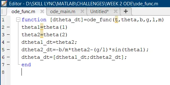
Here in this code we are implementing a concept called ‘function’, Where a function is a group of statements that together perform a task. In MATLAB, functions are defined in separate files. The name of the file and of the function should be the same.
Where dtheta_t is the matrix that we have derived in video
6.Now we have to call the function as follows

The output from the ode_fun will be stored in the [t,results],where ode_func is the name of the function
ode45 is a versatile ODE solver and is the first solver you should try for most problems. However, if the problem is stiff or requires high accuracy, then there are other ODE solvers that might be better suited to the problem
7.Where in results matrix there are 2 columns, where 1st Colum represents the Displacement and 2nd column represents the Angular velocity. Now we have to plot Time against these two using following commands
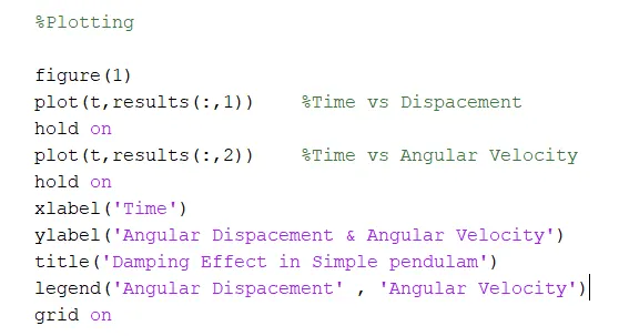
Using (:,1) we are selecting all the rows of an array and the first column
Using (:,2) we are selecting all the rows of an array and the second column
8.To result the animation of simple pendulum first we have to initialize the counter variable and we are implementing the for loop concept. Where value of I changes from the 1 to results(:,1) and using the calculation e have defined the initial and final postions of the pendulum
9.marker command is used to create the pendulum ball and in line 60 ct represents every frame and getframe command represents to getting the current figure in the gcf window. Further, we are going to save all the figures in the array called (M).
10.To create the AVI files following command are used
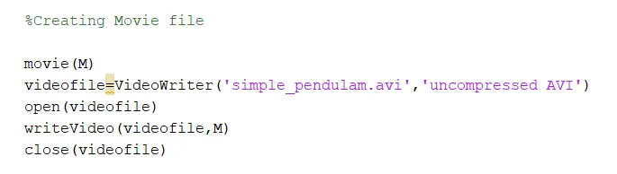
while using the writeVideo command we have to be carefull because MATLAB is case sensitive hence any mistake can give an error in the program execution
RESULT AND OBSERVATION:
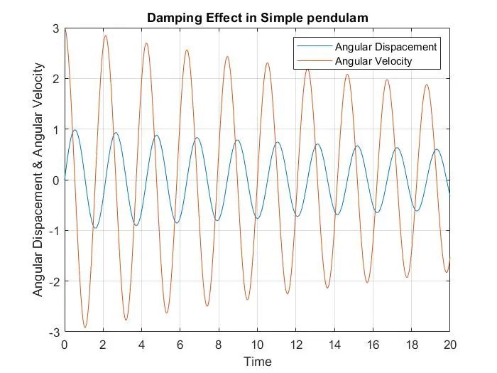
1.The curve of Angular displacement and Angular velocity is reducing with respect of time this is due to damping factor. When the motion of an oscillator reduces due to an external force, the oscillator and its motion are damped. These periodic motions of gradually decreasing amplitude are damped simple harmonic motion
ANIMATION LINK: https://youtu.be/abLsjNyv82s
ERRORS:
ERROR1:
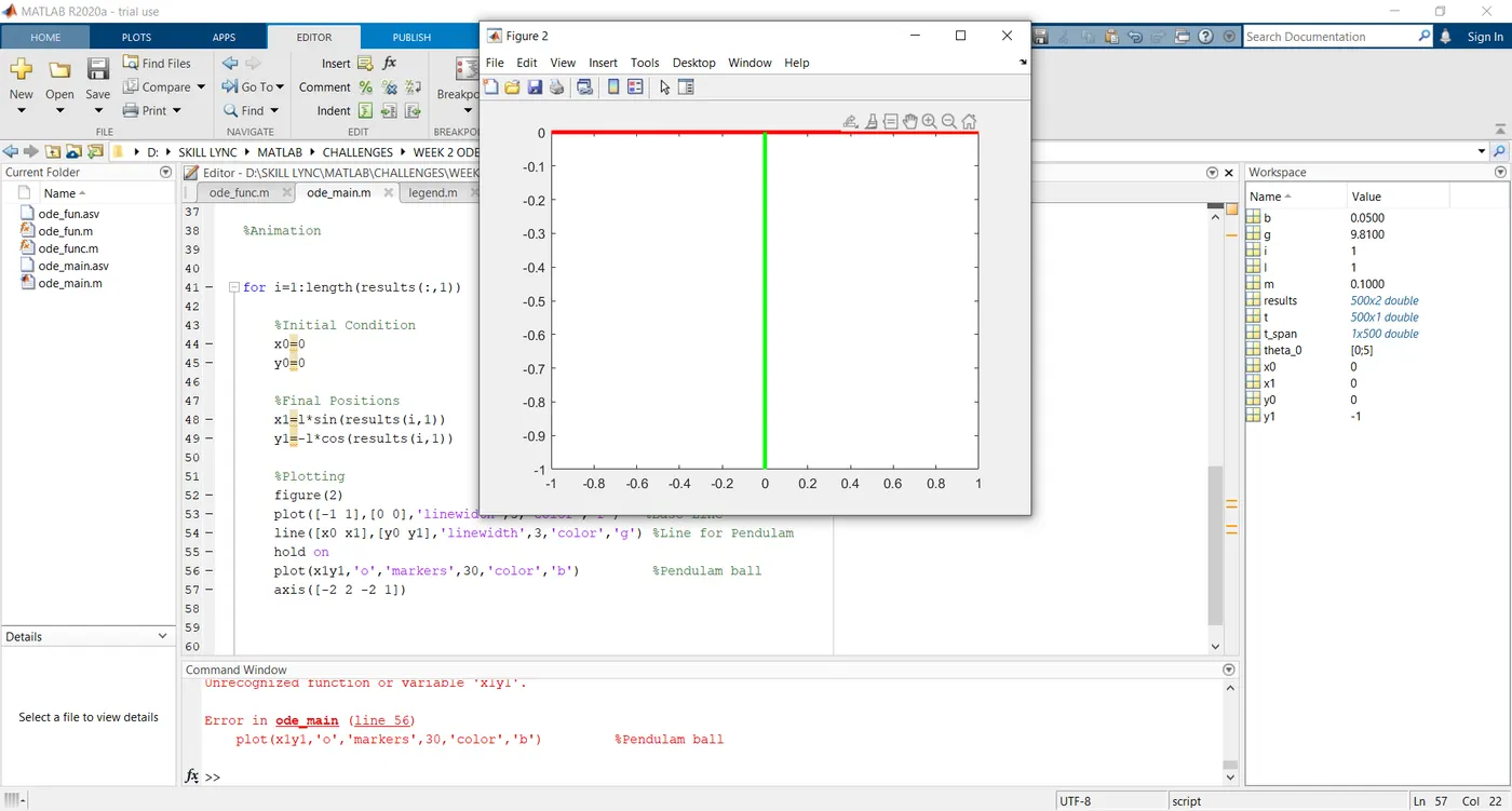
SOLUTION: After implementing the comma in line 56 between x1 and y1 the error got corrected
ERROR2:
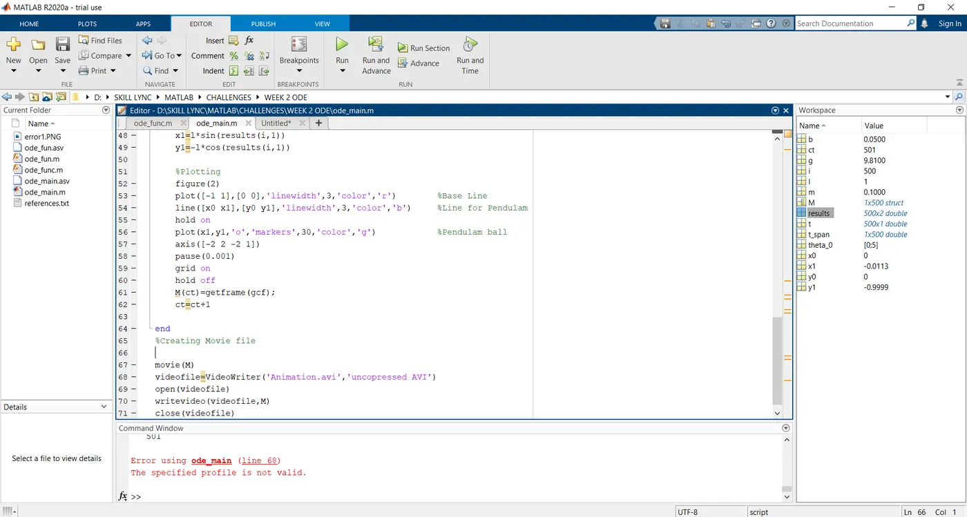
SOLUTION: The spelling of uncompressed Is wrong after correcting it its works properly
REFRENCES: