Study of Air standard Cycle using MATLAB
Air standard Cycle
OBJECTIVE:
We have to
- Code to create a PV diagram
- Output the thermal efficiencyof the engine.
THEORY:
The Otto cycle is a set of processes used by spark ignition internal combustion engines (2-stroke or 4-stroke cycles). These engines a) ingest a mixture of fuel and air, b) compress it, c) cause it to react, thus effectively adding heat through converting chemical energy into thermal energy, d) expand the combustion products, and then e) eject the combustion products and replace them with a new charge of fuel and air.
- Intake stroke, gasoline vapor and air drawn into engine (5-1)
- Compression stroke, P, T increase (1-2)
- Combustion (spark), short time, essentially constant volume (2-3) Model: heat absorbed from a series of reservoirs at temperatures T2 toT3 .
- Power stroke: expansion (3-4)
- Valve exhaust: valve opens, gas escapes.
- (4-1) Model: rejection of heat to series of reservoirs at temperatures T4 to T1 .
- Exhaust stroke, piston pushes remaining combustion products out of chamber (1-5)
We model the processes as all acting on a fixed mass of air contained in a piston-cylinder arrangement
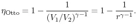
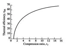
In terms of compression ratio, the efficiency of an ideal Otto cycle is:
MATLAB CODE:
CODE1:
%Simulating Air Standard Cycle


clear all
close all
clc

%State variables at point 1
p1=101325
t1=500

%Input Parameters
gamma=1.4
t3=2300

%Engine Geometric parameters
bore=0.1;
stroke=0.1;
con_rod=0.15;
cr=12;

%Calculating the swept volume and clearance volum
%Swept volume is the volume of cylinder

v_swept=(pi/4)*bore^2*stroke;
v_clearance=v_swept/(cr-1);
v1=v_swept+v_clearance
v2=v_clearance

%State variables at state point 2
%p2v2^gamma=p1v1^gamma
%p2=p1*(v1/v2)^gamma=p1*cr^gamma
p2=p1*cr^gamma

%p1v1/t1=p2v2/t2 | t2=p2*v2*t1/(p1*v1)
t2=p2*v2*t1/(p1*v1)


%State variable at state point 3
v3=v2

%p3v3/t3=p2v2/t2 | p3=p2*t3/t2
p3=p2*t3/t2


%State variable at point 4
v4=v1

%p3v3^gamma=p4v4^gamma  | p4=p3*(v3/v4)^gamma
p4=p3*(v3/v4)^gamma

%p4v4/t4=p3v3/t3  | t4=(p4*v4*t3)/(p3*v3)
t4=(p4*v4*t3)/(p3*v3)


%Plotting the PV diagram
figure(1)
hold on
plot(v1,p1,'*','color','r')
plot(v2,p2,'*','color','r')
plot(v3,p3,'*','color','r')
plot(v4,p4,'*','color','r')
xlabel('Volume')
ylabel('Pressure')
title('OTTO CYCLE')
CODE2:
%Engine Kinematics

function [V] =engine_kinematics(bore,stroke,con_rod,cr,start_crank,end_crank)

a=stroke/2;
R=con_rod/a;

v_swept=(pi/4)*bore^2*stroke;
v_c=v_swept/(cr-1);

theta=linspace(start_crank,end_crank,180)

term1=0.5*(cr-1);
term2=R+1-cosd(theta);
term3=(R^2-sind(theta).^2).^0.5;

V=(1+term1*(term2-term3)).*v_c


end
CODE3:
%Simulating Air Standard Cycle


clear all
close all
clc

%State variables at point 1
p1=101325
t1=500

%Input Parameters
gamma=1.4
t3=2300

%Engine Geometric parameters
bore=0.1;
stroke=0.1;
con_rod=0.15;
cr=12;

%Calculating the swept volume and clearance volum
%Swept volume is the volume of cylinder

v_swept=(pi/4)*bore^2*stroke;
v_clearance=v_swept/(cr-1);
v1=v_swept+v_clearance
v2=v_clearance

%State variables at state point 2
%p2v2^gamma=p1v1^gamma
%p2=p1*(v1/v2)^gamma=p1*cr^gamma
p2=p1*cr^gamma

%p1v1/t1=p2v2/t2 | t2=p2*v2*t1/(p1*v1)
t2=p2*v2*t1/(p1*v1)

constant_c=p1*v1^gamma
V_compression=engine_kinematics(bore,stroke,con_rod,cr,180,0)
P_compression=constant_c./V_compression.^gamma

%State variable at state point 3
v3=v2

%p3v3/t3=p2v2/t2 | p3=p2*t3/t2
p3=p2*t3/t2

constant_c=p3*v3^gamma
V_expansion=engine_kinematics(bore,stroke,con_rod,cr,0,180)
P_expansion=constant_c./V_expansion.^gamma

%State variable at point 4
v4=v1

%p3v3^gamma=p4v4^gamma  | p4=p3*(v3/v4)^gamma
p4=p3*(v3/v4)^gamma

%p4v4/t4=p3v3/t3  | t4=(p4*v4*t3)/(p3*v3)
t4=(p4*v4*t3)/(p3*v3)


%Plotting the PV diagram
figure(1)
hold on
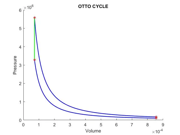
plot(V_compression,P_compression,'linewidth',1.5,'color','b')
plot(V_expansion,P_expansion,'linewidth',1.5,'color','b')
plot([v2 v3],[p2 p3],'linewidth',1.5,'color','g')
plot([v4 v1],[p4 p1],'linewidth',1.5,'color','g')
plot(v1,p1,'*','color','r')
plot(v2,p2,'*','color','r')
plot(v3,p3,'*','color','r')
plot(v4,p4,'*','color','r')
xlabel('Volume')
ylabel('Pressure')
title('OTTO CYCLE')


%Calculating the Thermal Efficiency
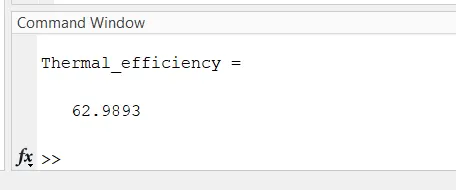
Thermal_efficiency=(1-(cr^(gamma-1))^-1)*100
EXPLANATION OF CODE:
We can divide the codes into 3
- CODE1
- CODE2
- CODE3
CODE1:
Clear all command used to clear text from the Command Window before running a command.
Close all command used to close all the plots window.
clc command is used to Clear Command Window
The input were given and state points were calculated implemented
For plotting, we are using plot command and we get a PV diagram having four-point in it which Represents State points.
The PV diagram with state points as follows
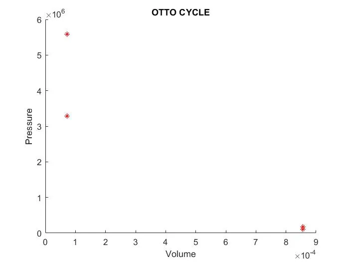
The CODE1 results this, we cannot join them by forming the lines because it is an isentropic process, So we have plot that correctly
To plot correctly, We have to use the Piston kinematics to determine How the volume change from TDC to BDC and how combustion volume changes as a function of the crank angle.
CODE2:
Here in this code we are implementing a concept called ‘function’, Where a function is a group of statements that together perform a task. In MATLAB, functions are defined in separate files. The name of the file and of the function should be the same.
Functions operate on variables within their own workspace, which is also called the local workspace, separate from the workspace you access at the MATLAB command prompt which is called the base workspace.
Functions can accept more than one input arguments and may return more than one output arguments.
Here we are taking same parameters but we need a different formula for the calculation, Following is the equation
V/Vc = 1+ 0.5(cr-10)* [ R+1 -cos(angle) — (R² -sin²(angle)⁰.5]
And we have to split the formula into term1, term2 and term3 for ease of calculation and after that we have to implement the defined function in our main code, the name of the function is engine_kinematics and we have to call this function by name in our main code
CODE3:
Now, in our main program, we are using this function for the Pressure and volume changes in the compression and Expansion stroke, for the volume we can define the function as follows.
V_expansion = engine_kinematics(bore,stroke,con_rod,cr,0,180);
But for the pressure, we know that P*V^gamma = constant_c
Hence, we are defining this relation and using it as, constant_c = P1*V1^gamma; and
P_compression = constant_c./V_compression.^gamma;
similarly, for Expansion, we are using the above relation as,
constant_c = P3*V3^gamma;
V_expansion = piston_kinematics(bore,stroke,con_rod,cr,180,0)
P_expansion = constant_c./V_expansion.^gamma;
And we have applied the function concept and now we have to plot the PV diagram.For that following commands were used
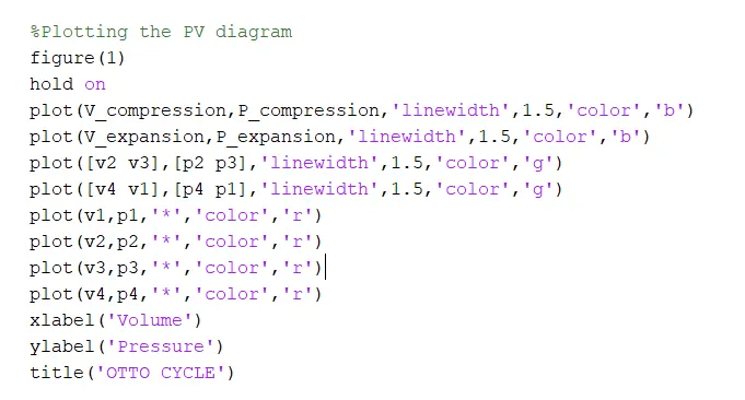
figure command creates a new figure object using default property values.
hold on retains the current plot and certain axes properties so that subsequent graphing commands add to the existing graph
The plot function in MATLAB is used to create a graphical representation of some data.
Finally we have to calculate the Thermal Efficiency of the engine using the formula
And we have calculated the thermal efficiency.
RESULT AND DISCUSSION:
PV DIAGRAM:
THERMAL EFFICIENCY:
FINAL:
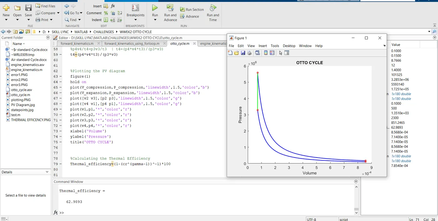
As per the requirement we have plotted the PV diagram and we have calculated the Thermal efficiency of the engine successfully
ERRORS FACED DURING THE CODING:
ERROR1:
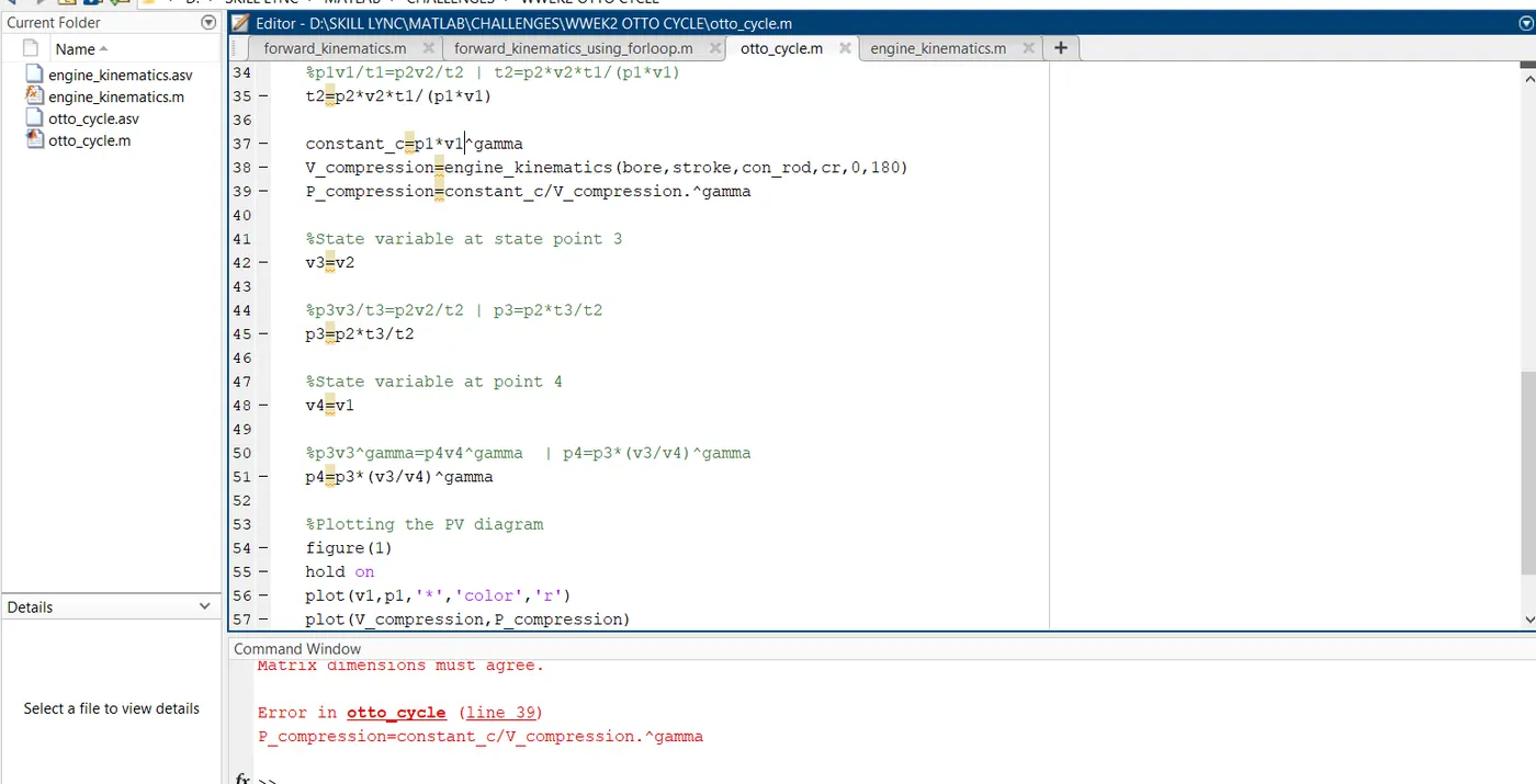
SOLUTION:
We have to use the dot operators because there is a vector operation is going on
ERROR2:
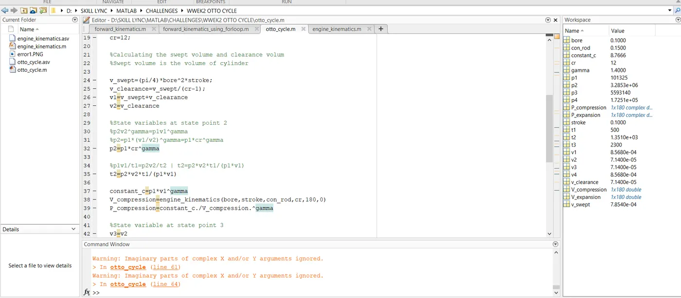
SOLUTION:
I have wrongly typed the equation in term2 of the function program that’s why this error happened and I have changed that and its works properly
REFERENCES:
- https://www.sciencedirect.com/topics/physics-and-astronomy/thermodynamic-analysis
- https://www.tutorialspoint.com/matlab/matlab_plotting.htm