Study of Curve fitting using MATLAB
Curve fitting
OBJECTIVE:
We have to
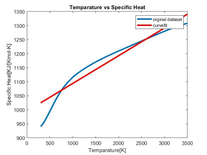
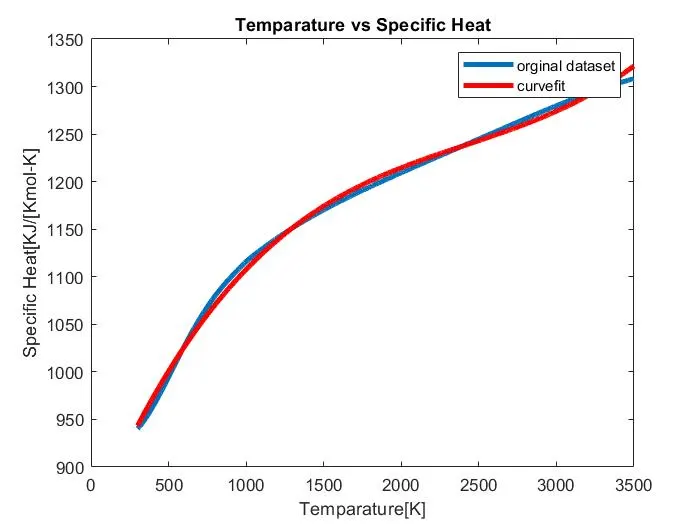
- Write code to fit a linear and cubic polynomial for the Cp data
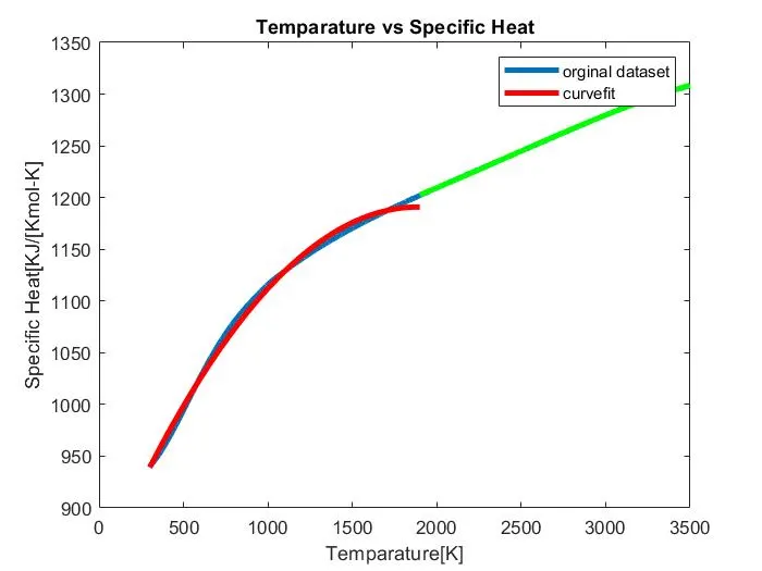
- Write a code to show splitwise method
- Explain the parameters used to measure the fitness characteristics for both the curves
- Use the Curve fitting toolbox in MATLAB to validate your fitness characteristics
THEORY:
Curve fitting is the process of constructing a curve, or mathematical functions, which possess
closest proximity to the series of data. By the curve fitting we can mathematically construct
the functional relationship between the observed fact and parameter values, etc. It is highly
effective in mathematical modelling some natural processes.
It is a statistical technique use to drive coefficient values for equations that express the value
of one(dependent) variable as a function of another (independent variable).
Why Curve Fitting?
The main purpose of curve fitting is to theoretically describe experimental data with a model
(function or equation) and to find the parameters associated with this model.
Mechanistic models are specifically formulated to provide insight into a chemical, biological or physical process that is thought to govern the phenomenon under study
It is important to distinguish mechanistic models from empirical models that are mathematical functions formulated to fit a particular curve but those parameters do not necessarily correspond to a biological, chemical or physical property
Evaluating the Goodness of Fit
After fitting data with one or more models, you should evaluate the goodness of fit. A visual examination of the fitted curve displayed in the Curve Fitting Tool should be your first step. Beyond that, the toolbox provides these goodness of fit measures for both linear and nonlinear parametric fits:
- Residuals
- Goodness of fit statistics
- Confidence and prediction bounds
You can group these measures into two types: graphical and numerical. The residuals and prediction bounds are graphical measures, while the goodness of fit statistics and confidence bounds are numerical measures.
Generally speaking, graphical measures are more beneficial than numerical measures because they allow you to view the entire data set at once, and they can easily display a wide range of relationships between the model and the data. The numerical measures are more narrowly focused on a particular aspect of the data and often try to compress that information into a single number. In practice, depending on your data and analysis requirements, you might need to use both types to determine the best fit.
Note that it is possible that none of your fits can be considered the best one. In this case, it might be that you need to select a different model. Conversely, it is also possible that all the goodness of fit measures indicate that a particular fit is the best one. However, if your goal is to extract fitted coefficients that have physical meaning, but your model does not reflect the physics of the data, the resulting coefficients are useless. In this case, understanding what your data represents and how it was measured is just as important as evaluating the goodness of fit.
Goodness of Fit Statistics
After using graphical methods to evaluate the goodness of fit, you should examine the goodness of fit statistics. The Curve Fitting Toolbox supports these goodness of fit statistics for parametric models:
The sum of squares due to error (SSE)
R-square
Adjusted R-square
Root mean squared error (RMSE)
For the current fit, these statistics are displayed in the Results list box in the Fit Editor. For all fits in the current curve-fitting session, you can compare the goodness of fit statistics in the Table of fits.
Sum of Squares Due to Error. This statistic measures the total deviation of the response values from the fit to the response values. It is also called the summed square of residuals and is usually labeled as SSE.
A value closer to 0 indicates a better fit. Note that the SSE was previously defined in The Least Squares Fitting Method.
R-Square. This statistic measures how successful the fit is in explaining the variation of the data. Put another way, R-square is the square of the correlation between the response values and the predicted response values. It is also called the square of the multiple correlation coefficient and the coefficient of multiple determination.
R-square is defined as the ratio of the sum of squares of the regression (SSR) and the total sum of squares (SST). SSR is defined as
SST is also called the sum of squares about the mean, and is defined as
where SST = SSR + SSE. Given these definitions, R-square is expressed as
R-square can take on any value between 0 and 1, with a value closer to 1 indicating a better fit. For example, an R2 value of 0.8234 means that the fit explains 82.34% of the total variation in the data about the average.
If you increase the number of fitted coefficients in your model, R-square might increase although the fit may not improve. To avoid this situation, you should use the degrees of freedom adjusted R-square statistic described below.
Note that it is possible to get a negative R-square for equations that do not contain a constant term. If R-square is defined as the proportion of variance explained by the fit, and if the fit is actually worse than just fitting a horizontal line, then R-square is negative. In this case, R-square cannot be interpreted as the square of a correlation.
Degrees of Freedom Adjusted R-Square. This statistic uses the R-square statistic defined above, and adjusts it based on the residual degrees of freedom. The residual degrees of freedom is defined as the number of response values n minus the number of fitted coefficients m estimated from the response values.
v indicates the number of independent pieces of information involving the n data points that are required to calculate the sum of squares. Note that if parameters are bounded and one or more of the estimates are at their bounds, then those estimates are regarded as fixed. The degrees of freedom is increased by the number of such parameters.
The adjusted R-square statistic is generally the best indicator of the fit quality when you add additional coefficients to your model.
The adjusted R-square statistic can take on any value less than or equal to 1, with a value closer to 1 indicating a better fit.
Root Mean Squared Error. This statistic is also known as the fit standard error and the standard error of the regression
where MSE is the mean square error or the residual mean square
PERFECT FIT: The “perfect fit' means when the curve goes through every point. The sum-of-squares is 0.0, and R^2 is 1.00.
BEST FIT: A RMSE value closer to 0 indicates a better fit.
MATLAB CODE:
For Linear Fit
%Performing Curvefit for linear polynomial

clear all
close all
clc


%Preparing the data

cp_data=load('data');           %Loading the file named data
temparature=cp_data(:,1);       %Genarating Temparature value from the data file
cp=cp_data(:,2);                %Genarating the cp value from the data file


%Curve Fitting
co_effec=polyfit(temparature,cp,1);  %Linear Polynomial f(T)=a*T+b,Value of coefficients a and b will stored in the array called co_effec
predicted_cp=polyval(co_effec,temparature); %Calculating the value of cp using the co_effecints and temparature value


%Plotting
%Comparing my ocurvefit with orginal data
plot(temparature,cp,'linewidth',3)
hold on
plot(temparature,predicted_cp,'linewidth',3,'color','r')
xlabel('Temparature[K]')'
ylabel('Specific Heat[KJ/[Kmol-K]')
title('Temparature vs Specific Heat')
legend('orginal dataset','curvefit')

%Determining Best Fit
n=3200 %Number of data points
error=(cp-predicted_cp)
SSE=sum(error.^2)
SSR=sum(cp-mean(cp)).^2
SST=SSE+SSR
R_Square=(SSR/SST)
RMSE=sqrt(SSE/n)
For Cubic Polynomial
%Performing Curvefit for cubic polynomial

clear all
close all
clc


%Preparing the data

cp_data=load('data');           %Loading the file namde data
temparature=cp_data(:,1);       %Genarating Temparature value from the data file
cp=cp_data(:,2);                %Genarating the cp value from the data file


%Curve Fitting
co_effec=polyfit(temparature,cp,3);  %cubic  Polynomial f(T)=a*T^3+b*T^2+c*T+d,Value of coefficients a,b,c and d  will stored in the array called co_effec
predicted_cp=polyval(co_effec,temparature); %Calculating the value of cp using the co_effecints and temparature value


%Plotting
%Comparing my ocurvefit with orginal data
plot(temparature,cp,'linewidth',3)
hold on
plot(temparature,predicted_cp,'linewidth',3,'color','r')
xlabel('Temparature[K]')'
ylabel('Specific Heat[KJ/[Kmol-K]')
title('Temparature vs Specific Heat')
legend('orginal dataset','curvefit')
Using Splitwise Method
%Performing curvefit
%Split Wise Method


clear all
close all
clc


%Preparing the data

cp_data=load('data');           %Loading the file namde data
temparature=cp_data(:,1);       %Genarating Temparature value from the data file
cp=cp_data(:,2);                %Genarating the cp value from the data file

%Curve fitting

%Assinging the splited values into arrays
TEMP1=temparature(1:1600)
CP1=cp(1:1600)
TEMP2=temparature(1600:3200)
CP2=cp(1600:3200)

co_effec1=polyfit(TEMP1,CP1,2);%Quadratic polynomial f(T)=a*T^2+b*T+c where coefficients a,b and c will be stored in th array
co_effec2=polyfit(TEMP2,CP2,3);%cubic Polynomial f(T)=a*T^3+b*T^2+c*T+d,Value of coefficients a,b,c,d will stored in the array

%predicted_cp
%Calculating the value of cp using the co_effecints and temparature value

predicted_cp1=polyval(co_effec1,TEMP1)
predicted_cp2=polyval(co_effec2,TEMP2)

%Plotting
%Comparing my ocurvefit with orginal data
plot(temparature,cp,'linewidth',3)
hold on
plot(TEMP1,predicted_cp1,'linewidth',3,'color','r')
plot(TEMP2,predicted_cp2,'linewidth',3,'color','g')
xlabel('Temparature[K]')
ylabel('Specific Heat[KJ/[Kmol-K]')
title('Temparature vs Specific Heat')
legend('orginal dataset','curvefit')
CODE EXPLANATION
1.Clear all command used to clear text from the Command Window before running a command.
Close all command used to close all the plots window.
clc command is used to Clear Command Window
2.Now we have to code to prepare the data, load command is used to open the file named data and then we have extracted the temperature and cp values separately
3.Polyfitis a MATLAB functionthat computes a least squares polynomial for a given set of data. Polyfit generates the coefficients of the polynomial, which can be used to model a curve to fit the data. For Linear Polynomial f(T)=a*T+b,Value of coefficients a and b will stored in the array called co_effec
4.For Cubic Polynomial f(T)=a*T^3+b*T^2+c*T+d,Value of coefficients a,b,c and d will stored in the array called co_effec
5.While performing Split wise method we have to create two separate arrays for temperature and cp,After that we have to store the values of co-efficient separately, For Quadratic polynomial f(T)=a*T^2+b*T+c where coefficients a,b and c will be stored in the array and cubic Polynomial f(T)=a*T^3+b*T^2+c*T+d,Value of coefficients a,b,c,d will stored in the array called co_effec1 and co_effec2
Polyval evaluates a polynomial for a given set of x values. So, Polyval generates a curve to fit the data based on the coefficients found using polyfit.
6.Now next part of the section is plotting we have to plot temperature against predicted_cp and temperature against cp
legend (MATLAB Functions) legend places a legend on various types of graphs (line plots, bar graphs, pie charts, etc.). For each line plotted, the legend shows a sample of the line type, marker symbol, and color beside the text label you specify.
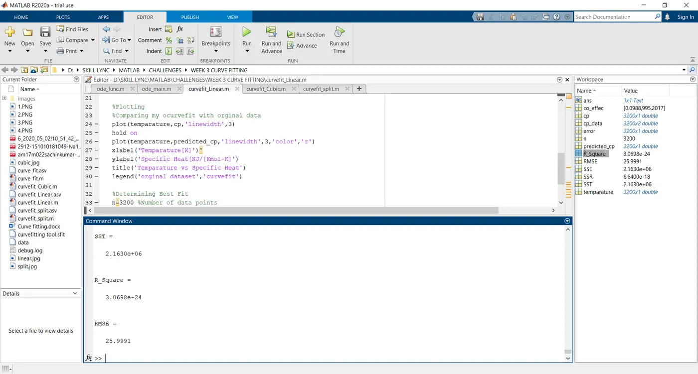
7.Now we have to determine the Best fit,By using the above equation we have calculated the error,SSE,SSR,SST,R_SQUARE,RMSE
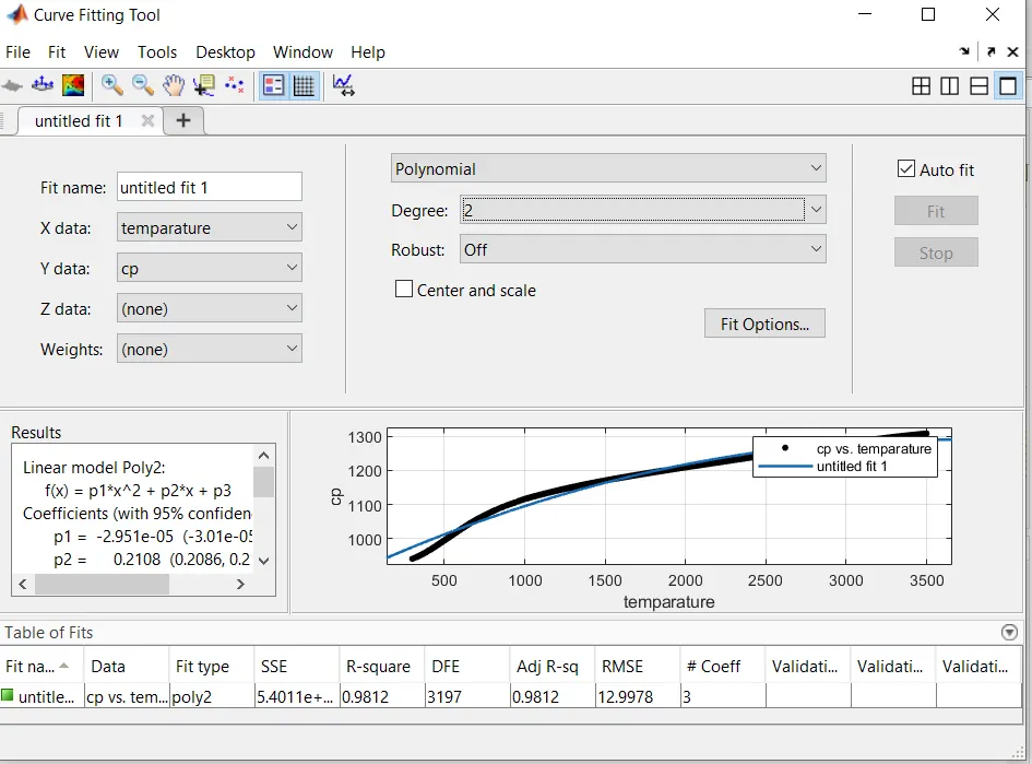
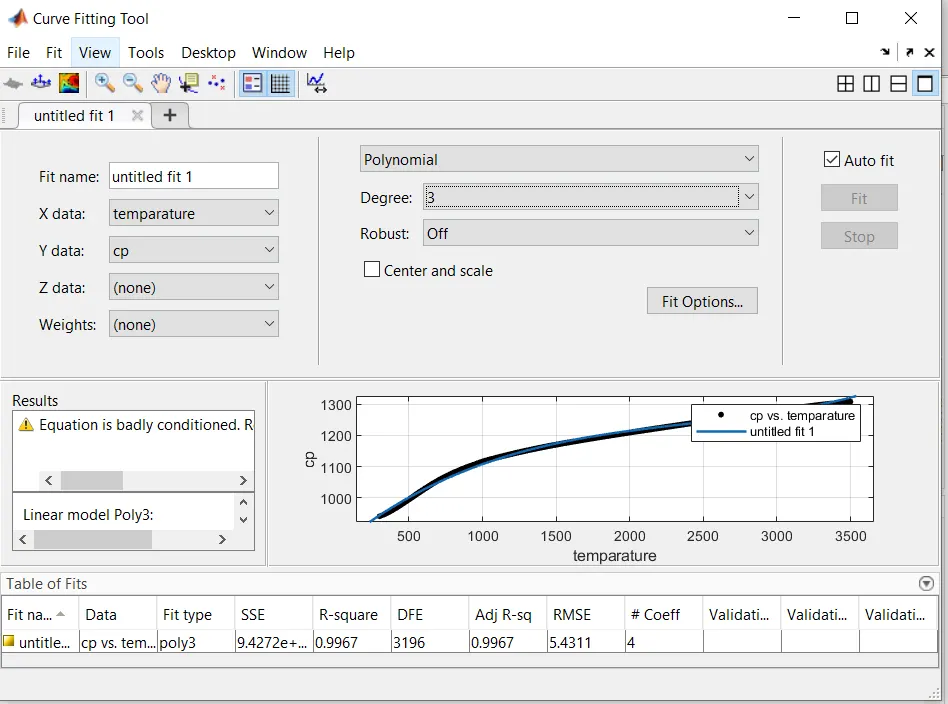
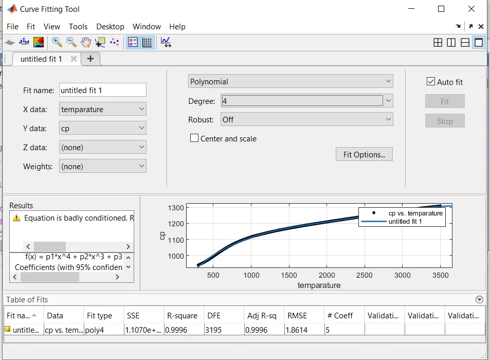
8.And to validate the fitness characteristics we have used the curvefitting toolbox in MATLAB, The results is attaching in the results
RESULTS AND OBSERVATIONS:
Curve fit for Linear Polynomial:
Curve fit for cubic Polynomial:
Split Wise Method:
RESULTS OF CURVEFITTING TOOL UPTO 4 DEGREE:
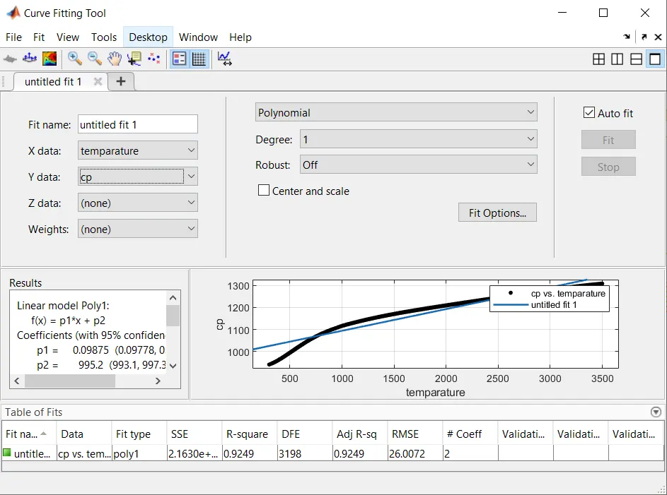
RESULT OF FIT CALCULATION:
OBSERVATION:
R-square can take on any value between 0 and 1, with a value closer to 1 indicating a better fit. For example, an R2 value of 0.8234 means that the fit explains 82.34% of the total variation in the data about the average.
If you increase the number of fitted coefficients in your model, R-square might increase although the fit may not improve.
A RMSE value closer to 0 indicates a better fit.
REFRENCEES: