Study to calculate the calculate drag force against a cyclist using MATLAB

Flow over Bicycle

OBJECTIVE:

WE have to

• Write a MATLAB program to calculate drag force against a cyclist.
• Write a program to plot Velocity vs Drag force
• Write a program to plot Drag Co-efficient vs Drag force

THEORY:

A drag force is the resistance force caused by the motion of a body through a fluid, such as water or air. A drag force acts opposite to the direction of the oncoming flow velocity. This is the relative velocity between the body and the fluid.

The drag force D exerted on a body traveling through a fluid is given by

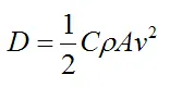
Where:

C is the drag coefficient, which can vary along with the speed of the body. But typical values range from 0.4 to 1.0 for different fluids (such as air and water)

ρ is the density of the fluid through which the body is moving

v is the speed of the body relative to the fluid

A is the projected cross-sectional area of the body perpendicular to the flow direction (that is, perpendicular to v).

NOTE: In our code Drag coefficient is represented by c_d and Drag force is represented by drag force

PROGRAM:

MATLAB Code to calculate the Drag force and plot Velocity VS Drag Force

%Program to Calculate the Drag force and  plot Velocity vs Dragforce

clear all
close all
clc

%Basic Inputs

rho=1.2  %Density(Kg/m^3)
A=0.1    %Area(m^2)
V=[1:50] %Velocity(m/s)
c_d=0.8  %Drag Coefficient(Non dimensional Quantity)

%Calculation
drag_force=rho*A*V.^2*c_d*0.5

%Plotting
plot(V,drag_force)
xlabel('Velocity(m/s)')
ylabel('Drag foce(Kgm/s)')
title('Velocity VS Dragfoce')
grid on 

MATLAB code to Calculate the Drag force and plot Drag coefficient vs Drag force

%Program to Calculate the Dragforce and  plot Dragcoefficient vs Dragforce

clear all
close all
clc

%Basic Inputs

rho=1.2                    %Density(Kg/m^3)
A=0.1                      %Area(m^2)
V=10                       %Velocity(m/s)
c_d=[0.1,0.2,0.3,0.4,0.5]  %Drag Coefficient(Non dimensional Quantity)

%Calculation
drag_force=rho*A*V.^2*c_d*0.5

%Plotting
plot(c_d,drag_force)
xlabel('Drag Coefficient(Non dimensional Quantity)')
ylabel('Dragfoce(Kgm/s)')
title('Drag Coefficient VS Dragfoce')
grid on 

EXPLANATION:

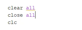
clear all, close all, clc; This clears your workspace, closes all figures, and clears command window.

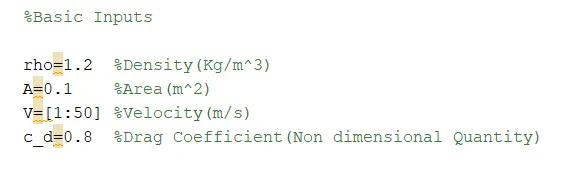
In this we have defined our inputs to calculate the Drag force and we have created an array for Velocity where the values of velocity varies from 1 to 50.

‘:’ Range operator is used to define the starting value and ending value of Velocity

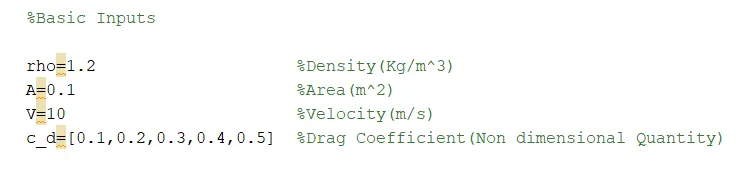
Here we have created the values of drag coefficient as an array

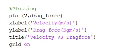
Plotting can be done using the command plot,We can give the representations of X axis and Y axis using the xlabel and ylabel command

To give title for the plot we have used the title command and grid command is to show the grid on the plots

RESULTS:

CONCLUSION:

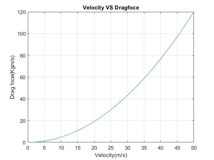
As we can see in first output that, Increase in velocity result increase in Drag force exponentially This is the disadvantage of the cyclist and to overcome this we have to reduce the frontal area.

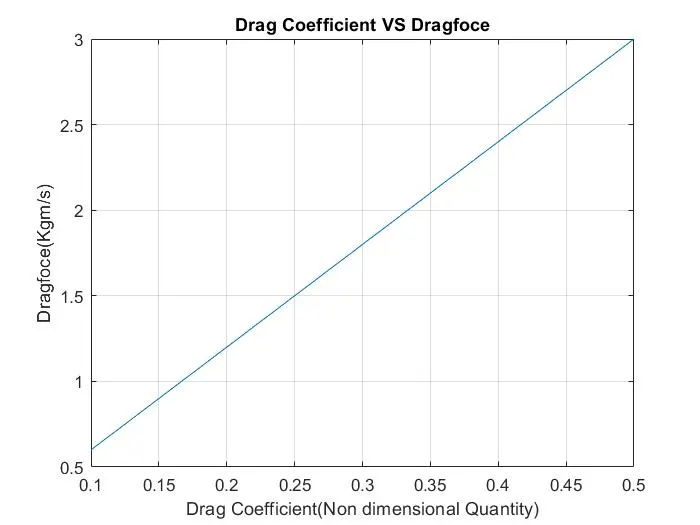
As we can see in the second output that Drag force is directly proportional to the Drag coefficient