Program for curve fitting

AIM:

Theory: Curve fitting is the process of constructing a curve, or mathematical function, that has the best fit to a series of data points, possibly subject to constraints.

QUESTIONS:

1. What does popt and pcov mean?

ANS:”popt’ is an array where in this case it will store the values of coeficients

:”pcov” is an 2D array that contains estimated covariance of popt

2. What does np.array(temperature) do?

ANS:This code will convert the list of trmparture to a numpy array

3. What does the * in *popt mean?

ANS:The above command to store values of coefficinets in popt array

4. Write code to fit a linear and cubic polynomial for the Cp data

#PROGRAM TO PERFORM CURVE FITTING FOR LINEAR FUNCTION

#PROGRAM TO PERFORM CURVE FITTING FOR LINEAR FUNCTION


import math
import matplotlib.pyplot as plt
import numpy as np
from scipy.optimize import curve_fit


def function(t,a,b):
	return a*t+b

def read_file():
	temp=[]
	cp=[]
	for line in open('data' , 'r'):
		values=line.split(',')
		temp.append(float(values[0]))
		cp.append(float(values[1]))

	return[temp,cp]


#Main Program

temp,cp=read_file()
popt,pcov=curve_fit(function,temp,cp)
fit_cp=function(np.array(temp),*popt)



#PLOTTING

	
plt.plot(temp,cp,color="red",linewidth=3)
plt.plot(temp,fit_cp,color="blue",linewidth=3)
plt.legend(['actual data', 'curve fit data'])
plt.xlabel('temparature[k]')
plt.ylabel('cp')
plt.show()

RESULT:

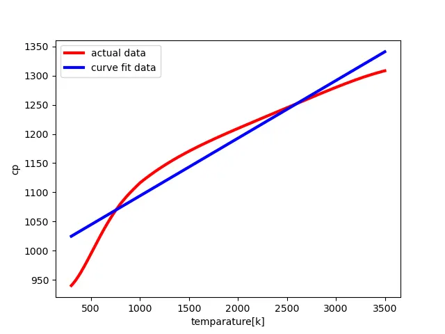
For cubic polynominial :

#PROGRAM TO PERFORM CURVE FITTING FOR CUBIC POLYNOMIAL

import math
import matplotlib.pyplot as plt
import numpy as np
from scipy.optimize import curve_fit


def function(t,a,b,c,d):
	return a*pow(t,3)+b*pow(t,2)+c*t+d

def read_file():
	temp=[]
	cp=[]
	for line in open('data' , 'r'):
		values=line.split(',')
		temp.append(float(values[0]))
		cp.append(float(values[1]))

	return[temp,cp]


#Main Program

temp,cp=read_file()
popt,pcov=curve_fit(function,temp,cp)
fit_cp=function(np.array(temp),*popt)



#PLOTTING

	
plt.plot(temp,cp,color="red",linewidth=3)
plt.plot(temp,fit_cp,color="blue",linewidth=3)
plt.legend(['actual data', 'curve fit data'])
plt.xlabel('temparature[k]')
plt.ylabel('cp')
plt.show()

RESULT:

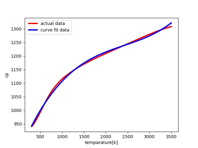
EXPLANATION OF CODE:

If we consider both cases the on;y difference is the functions that we defined.As you can see by using “from scipy.optimize import curve_fit” this code we are importing the curvefit function from scipy module.We have define the functions,As you can see the command “for line in open('data' , 'r'):” were it will open the file named data and the letter ‘r’ represent to read the the file.In next line the temparture and specific heat values will assingn to respective arrays that we have already created the empty arrays for both,Where the ‘append’ command is used to add the values into the respective arrays.Finally we will return the arrays.

As you can see in the main program ‘popt’ and ‘pcov’,where popt where in this case it will store the values of coeficients and the pcov is an 2D array that contains estimated covariance of popt.and ‘np’ command is to call the numpy module.and using the ‘plt.plot’ command we are going to plot both curves.

5.What needs to be done in order to make the curve fit perfect?

ANS:If we increase the polynomial order we will be reducing the error and mostly we will be getting perfect curves

CONCLUSION:

The observation that we got during this coding is ,If we increase the polynomial order we will be reducing the error and mostly we will be getting perfect curves