Week 3 - Solving second order ODEs

Aim: To Write a program in Matlab that will simulate the pendulum motion using the given values

Given values:
L=1 metre,
m=1 kg,
b=0.05,
g=9.81 m/s2,
The motion of the pendulum between 0-20 sec,
Angular displacement=0,
Angular velocity=3 rad/sec at time t=0.

Requirments:

• For each value in time
• Create an image that represents the position of the pendulum
• You can assume the length of the string and the size of the ball
• Use the marker command to create a sphere
• One end of the pendulum is fixed
• The other end moves according to the solution of the ODE you had solved.
• Use the movie command create an animation

Theory:

Introduction: ODe is extremily importent in engineering feald
They describes a lote of importent information & solving this ODE helps us to understand the system

Examples that involves in ODE are 1) simple pendulum
2)It also able to discrib motion of a spring mass and damper system, The same ODE used to describe Application in vechile dynamics you can also figure out how your vechile dynamics is going to be.

FUNCTION CODE:

function [dtheta_dt] = ode_func(t, theta, b, g, l, m)
theta1 = theta(1)
theta2 = theta(2)

dtheta1_dt = theta2;
dtheta2_dt = -(b/m)*theta2-(g/l)*sin(theta1);
dtheta_dt = [dtheta1_dt;dtheta2_dt];

MAIN CODE:

%code 
clear all
close all
clc
%taking inputs
b = 0.05;%damping co-efficent
g = 9.81;% gravity
l = 1; %length of the pendulam in m/s
m = 1;%mass

%defining inetial conditions 
theta_0 = [0,3];
%time points
t_span = linspace(0,20,300);

%solving ODE 
[t,results] = ode45(@(t,theta) ode_func(t,theta,b,g,l,m),t_span,theta_0);

%ploting
figure(1)
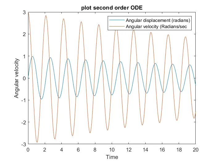
plot(t,results(:,1)) % to plot the column 1
hold on % to hold the figure
plot(t,results(:,2)) % to plot the column 2
hold off %to stop the hold on
xlabel('Time') %labling in graph on x-axis
ylabel('Angular velocity')%labling in graph on y-axis
title('plot second order ODE')% giving the title for the graph
legend('Angular displacement (radians)','Angular velocity (Radians/sec')%to specify the type of lines 

ct=1
%starting the function
for i = 1:length(t) 
x = l*sin(results(i,1)); %Giving the x value
y = -1*cos(results(i,1));%Giving the y value

figure(2)
plot([-0.4 0.4],[0 0],'linewidth',4,'color','g') %for ploting the fixed line
hold on
plot(x,y,'Marker','O','MarkerEdgeColor','red','MarkerFaceColor',[1 .6 .6],'Markersize',15) %to plot the bob size and color

plot([0 x],[0,y],'linewidth',1.5,'color','b') % To plot the rope of the bob
plot(0,0,'-o','MarkerFaceColor','k','MarkerSize',5) %fixed point of the rope
hold off

xlabel('x axis') %labling in graph on x-axis
ylabel('y axis')%labling in graph on y-axis
title('Simulation f simple pendulum') % giving title for the graph
axis([-3 3 -3 3])% giving area for the graph
legend('fixed line','bob','rope','connectin b/w rope and fixed line')%to specify the type of lines 

pause(0.03) % to slow the reel
M(ct) = getframe(gcf) % to make the frames
ct=ct+1; % to add the frame
end % to end the function
  % To create movie
  movie(M)
  % To give file name and formate
  videofile = VideoWriter('Simulation of a simple pendulum.avi','uncompressed AVI');
  % To open video
  open(videofile)
  % To make the plots togather and frame
  writeVideo(videofile,M)
  % To close the video
  close(videofile)
  
  
  
    

Explanation:

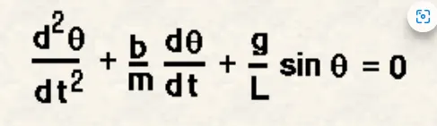
The following second order ODE represent the equation of a simple pendulum with damping

As per above equation
g = Accleration due to gravity in m/s2
l = length of the pendulum in m
m = mass of the pendulum in kg
b = damping co-efficient.

step wise explanation of the code:

step 1) split the above second order equation in to two first order equations & write the function code with a vailable colled [dtheta_dt] and function name is ode_func and inpus are temperature,theta,drag coficient,gravity,length of thread,mass of the bob

step 2) Lets make theta1=theta(1) & theta2=theta(2) Then give the 2 first order ODES
dtheta1_dt & dtheta2_dt and then make the matrix of both by assigning the veriable called dtheta_dt & save the file

Step 3) Come to main program & start the program in matlab with clear the privious calculations,to do that we have 3 commonds
clear all : To clear the work space priviously,
close all : To close the plots priviously,
clc : To clear the command window.

Step 4) Give the input values which are given in question that is Damping co-efficent , gravity, length of the pendulum, & mass of bob

Step 5)Defining inetial conditions of the pendulum with Displacement, Velocity by assigning the veriable colled theta_0

Step 6) To intigrate ode system to get values i am using time intervels for the motion of pendulum t_span is a time array it gows from 0 to 20 second with 300 values in bitween

Step 7) Then Call our ode function by using inbuild solver ode45 is a function of (t,theta) then provide input conditions, time_span, theta_0 which is initial conditions

Step 8) sins we solving two ode's and reasults to be column vector in specific we have two column vector figure(1)
plot(t,results(:,1)) to plot the first column which is displacement hold on to hold the plot & then plot(t,results(:,2))
plot the second column which is velocity hold off to stop hold on
Then lable the graph of x-axis and y-axis, give the title name & legend to specify line.

Step 9) To make a For loop and to creat an animation we need to use M(ct) where ct is the counter vereable which is given above , To apply a loop to change of desplay with displacement with respect to time

And by using pitogarus therom we cen able to get x & y values to get positions of the two points fixed and moving point

Step 10)figure2 write the code for ploting the fixed line by giving x & y positions in graph with a linewidth 4 and color green & write hold on to hold the privious plot

Step 11) On the other end,plot the bob by using marker command and give the size . Then join the fixed line which is (0,0) and bob with a rope line by giving length and thickness of the rope then hold off to stop the hold on command and then lable the axis, give the title,give the graph area by using the code axis(-x x ,-y y) & give the legend to represent the lines

step 12)Now to creat an animation we need to use M(ct) = getframe(gcf) where ct is the counter vereable
for incriment of the frame '1' is added
now to assigne the file name and file formate in .AVI. VideoWriter command is used. and to open the video file open(videofile) command is used And to write the vide with plot frame writerVideo command is used and to close the video close(videofile) command is used

step 13) After the program is don. click the run button or F5 shortcut on keybord to run the command then it will run the command and displays the animation and then the video and then the video is going to save on the file in which the program file path is alredy saved

The following 2. Errors that i faced wile programing:

ERROR-1. I wrote sind(theta1) insted of sin(theta1) in the function code and the error that i faced is

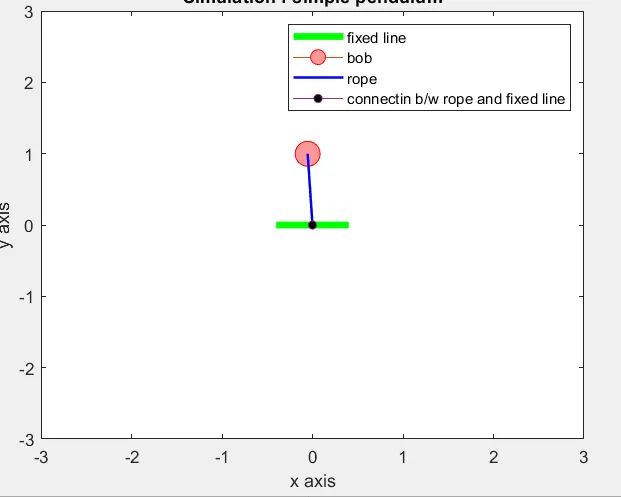The bob revolves around with the fixed point more then 360 digris

Later i found the mistake that i faced and then rectified it.

ERROR-2. To defining inetial conditions theta_0 = [0,3] Insted i put colon in bitween the values=[0:3] and i got the arror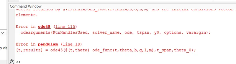Later i replaced it with cama ','

ERROR-3 The error that i got becose of not putting hold off command after ploting so that i got the reasult was multipul frames togather with a single image

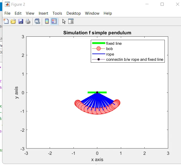later i do rectified by adding hold off command then i got my reasult